Challenge Importance

The time has come to add another layer to the hierarchy of Machine Learning models.

Do we have the variable we want to predict in the dataset?

YES: Supervised Learning

• Predicting a Numerical Variable → Regression

• Predicting a Categorical Variable → Classification

NO: Unsupervised Learning

• Group Data Points based on Explanatory Variables → Cluster Analysis

We may have, for example, all football players, and we want to group them based on their performance. But we don't know the groups beforehand. So what do we do then?

We apply Unsupervised Machine Learning models to group the players based on their position in the space (determined by the explanatory variables): the closer the players are to the space, the more likely they'll be drawn to the same group.

Another typical example comes from e-commerces that don't know if their customers like clothing or tech. But they know how they interact on the website. Therefore, they group the customers to send promotional emails that align with their likes.

In short, we close the circle with the different types of Machine Learning models by adding this new type.

Let's now develop the Python code.

Load the Data

Imagine for a second you are the President of the United States of America, and you are considering creating campaigns to reduce car accidents due to alcohol consumption controlling the impact of insurance companies' losses (columns).

You won't create 51 TV campaigns for each of the States of the USA (rows). Instead, you will see which States behave similarly to cluster them into three groups.

import seaborn as sns #!
import pandas as pd

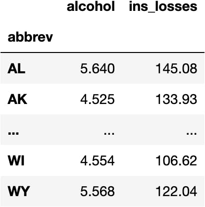
df_crashes = sns.load_dataset(name='car_crashes', index_col='abbrev')[['alcohol', 'ins_losses']]
df_crashes

Data Preprocessing

Missing Data

We don't have any missing data in any of the columns:

df_crashes.isna().sum()

alcohol 0 ins_losses 0 dtype: int64

Dummy Variables

Neither we need to convert categorical columns to dummy variables because the two we are considering are numerical.

df_crashes

How do we compute a k-Means Model in Python?

We should know from previous chapters that we need a function accessible from a Class in the library sklearn.

Import the Class

from sklearn.cluster import KMeans

Instantiante the Class

Create a copy of the original code blueprint to not "modify" the source code.

model_km = KMeans()

Access the Function

The theoretical action we'd like to perform is the one we executed in previous chapters. Therefore, the function to compute the Machine Learning model should be called the same way:

model_km.fit()

---------------------------------------------------------------------------

TypeError Traceback (most recent call last)

Input In [6], in <cell line: 1>() ----> 1 model_km.fit()

TypeError: fit() missing 1 required positional argument: 'X'

The previous types of models asked for two parameters:

• y: target ~ independent ~ label ~ class variable

• X: explanatory ~ dependent ~ feature variables

Why is it asking for just one parameter now, X?

As we said before, this model (unsupervised learning) doesn't know how the groups are calculated beforehand; they know after we compute the Machine Learning model. Therefore, they don't need to see the target variable y.

Separate the Variables

We don't need to separate the variables because we have explanatory ones.

Fit the Model

model_km.fit(X=df_crashes)

KMeans()

Predictions

Calculate Predictions

We have a fitted KMeans. Therefore, we should be able to apply the mathematical equation to the original data to get the predictions:

model_km.predict(X=df_crashes)

array([7, 3, 0, 7, 6, 7, 6, 1, 3, 7, 7, 5, 4, 7, 0, 5, 3, 3, 2, 4, 2, 3, 1, 3, 1, 7, 4, 5, 7, 5, 1, 5, 1, 3, 0, 3, 6, 0, 1, 1, 5, 4, 1, 1, 0, 0, 1, 0, 1, 0, 5], dtype=int32)

We wanted to calculate three groups, but Python is calculating eight groups. Let's modify this hyperparameter of the KMeans model:

model_km = KMeans(n_clusters=3)
model_km.fit(X=df_crashes)
model_km.predict(X=df_crashes)

array([0, 0, 1, 0, 2, 0, 2, 0, 0, 0, 0, 1, 1, 0, 1, 1, 0, 0, 2, 1, 2, 0, 0, 0, 0, 0, 1, 1, 0, 1, 0, 1, 0, 0, 1, 0, 2, 1, 0, 0, 1, 1, 0, 0, 1, 1, 0, 1, 0, 1, 1], dtype=int32)

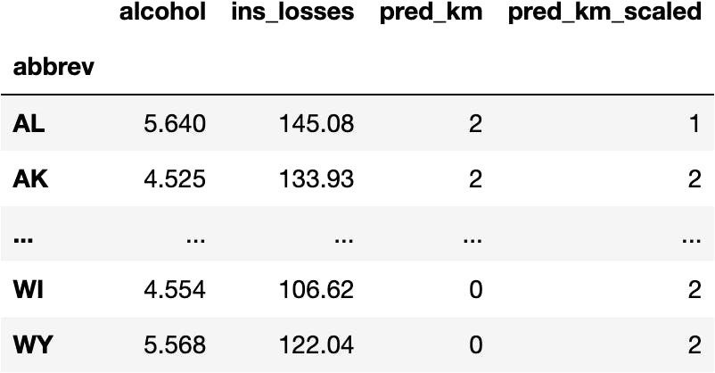
Add a New Column with the Predictions

Let's create a new DataFrame to keep the original dataset untouched:

df_pred = df_crashes.copy()

And add the predictions:

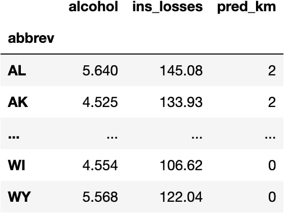
df_pred['pred_km'] = model_km.predict(X=df_crashes)
df_pred

How can we see the groups in the plot?

Model Visualization & Interpretation

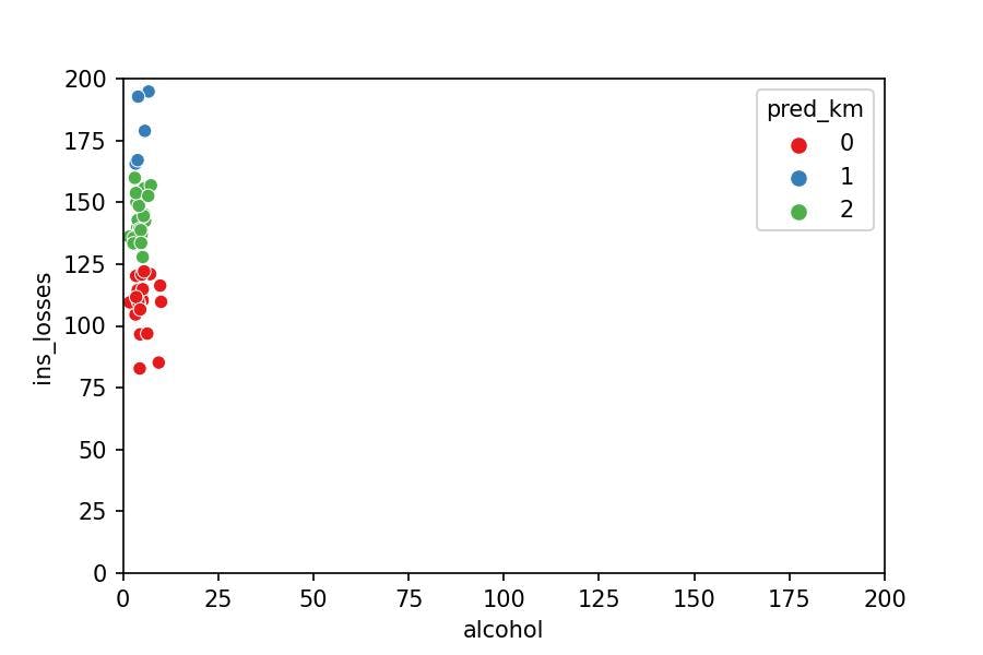
Can you observe that the k-Means only considers the variable ins_losses to determine the group the point belongs to? Why?

sns.scatterplot(x='alcohol', y='ins_losses', hue='pred_km',
                palette='Set1', data=df_pred);

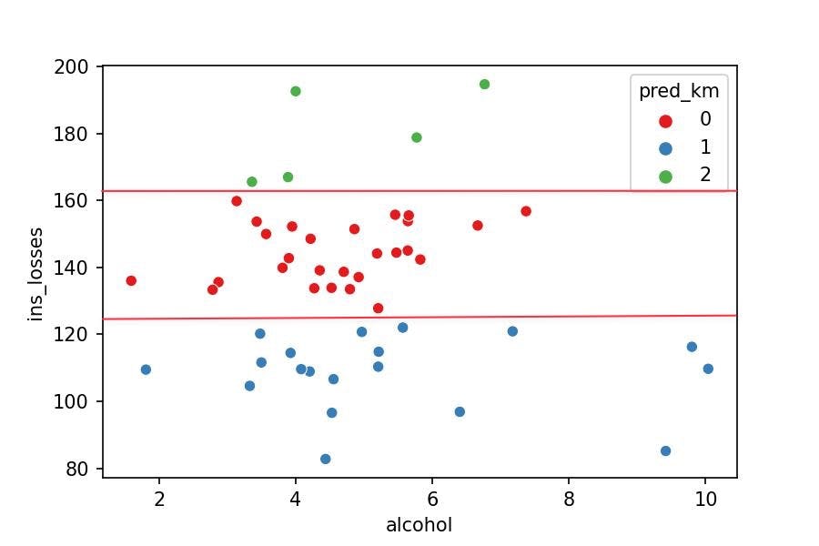
The model measures the distance between the points. They seem to be spread around the plot but aren't; the plot doesn't place the points in perspective (it's lying to us).

Learn how to become an independent Machine Learning programmer who knows when to apply any ML algorithm to any dataset.

KMeans Algorithm

Take a look at the following video to understand how the KMeans algorithm computes the Mathematical Equation by calculating distances:

The model understands the data as follows:

import matplotlib.pyplot as plt

sns.scatterplot(x='alcohol', y='ins_losses', hue='pred_km',
                palette='Set1', data=df_pred)
plt.xlim(0, 200)
plt.ylim(0, 200);

Now it's evident why the model only took into account ins_losses: it barely sees significant distances within alcohol compared to ins_losses.

In other words, with a metaphor: it is not the same to increase one kg of weight than one meter of height.

Then, how can we create a KMeans model that compares the two variables equally?

• We need to scale the data (i.e., transforming the values into the same range: from 0 to 1) with the MinMaxScaler.

MinMaxScaler() the data

As with any other algorithm within the sklearn library, we need to:

1. Import the Class

2. Create the instance

3. fit() the numbers of the mathematical equation

4. predict/transform the data with the mathematical equation

from sklearn.preprocessing import MinMaxScaler

scaler = MinMaxScaler()
scaler.fit(df_crashes)
data = scaler.transform(df_crashes)
data[:5]

array([[0.47921847, 0.55636883], [0.34718769, 0.45684192], [0.42806394, 0.24636258], [0.50100651, 0.5323574 ], [0.20923623, 0.73980184]])

To better understand the information, let's convert the array into a DataFrame:

df_scaled = pd.DataFrame(data, columns=df_crashes.columns, index=df_crashes.index)
df_scaled

k-Means Model with Scaled Data

Fit the Model

model_km.fit(X=df_scaled)

KMeans(n_clusters=3)

Predictions

Calculate Predictions

We have a fitted KMeans. Therefore, we should be able to apply the mathematical equation to the original data to get the predictions:

model_km.predict(X=df_scaled)

array([1, 0, 0, 1, 1, 1, 1, 1, 0, 1, 1, 2, 0, 1, 0, 0, 0, 1, 1, 0, 1, 0, 1, 0, 1, 1, 2, 0, 1, 0, 1, 0, 1, 0, 2, 0, 1, 0, 1, 1, 2, 2, 1, 1, 0, 0, 1, 0, 1, 0, 0], dtype=int32)

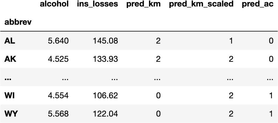
Add a New Column with the Predictions

df_pred['pred_km_scaled'] = model_km.predict(X=df_scaled)
df_pred

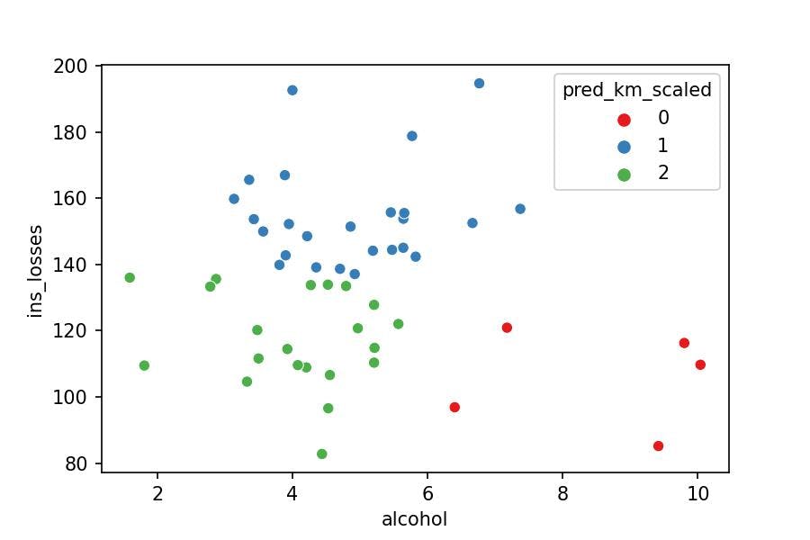
Model Visualization & Interpretation

We can observe now that both alcohol and ins_losses are taken into account by the model to calculate the cluster a point belongs to.

sns.scatterplot(x='alcohol', y='ins_losses', hue='pred_km_scaled',
                palette='Set1', data=df_pred);

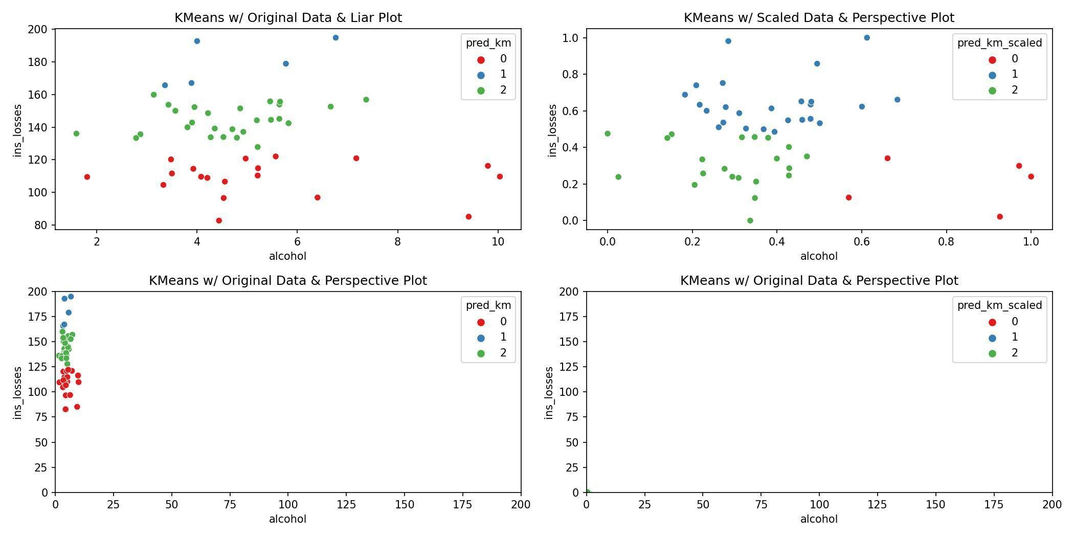
Takeaway

From now on, we should understand that every time a model calculates distances between variables of different numerical ranges, we need to scale the data to compare them properly.

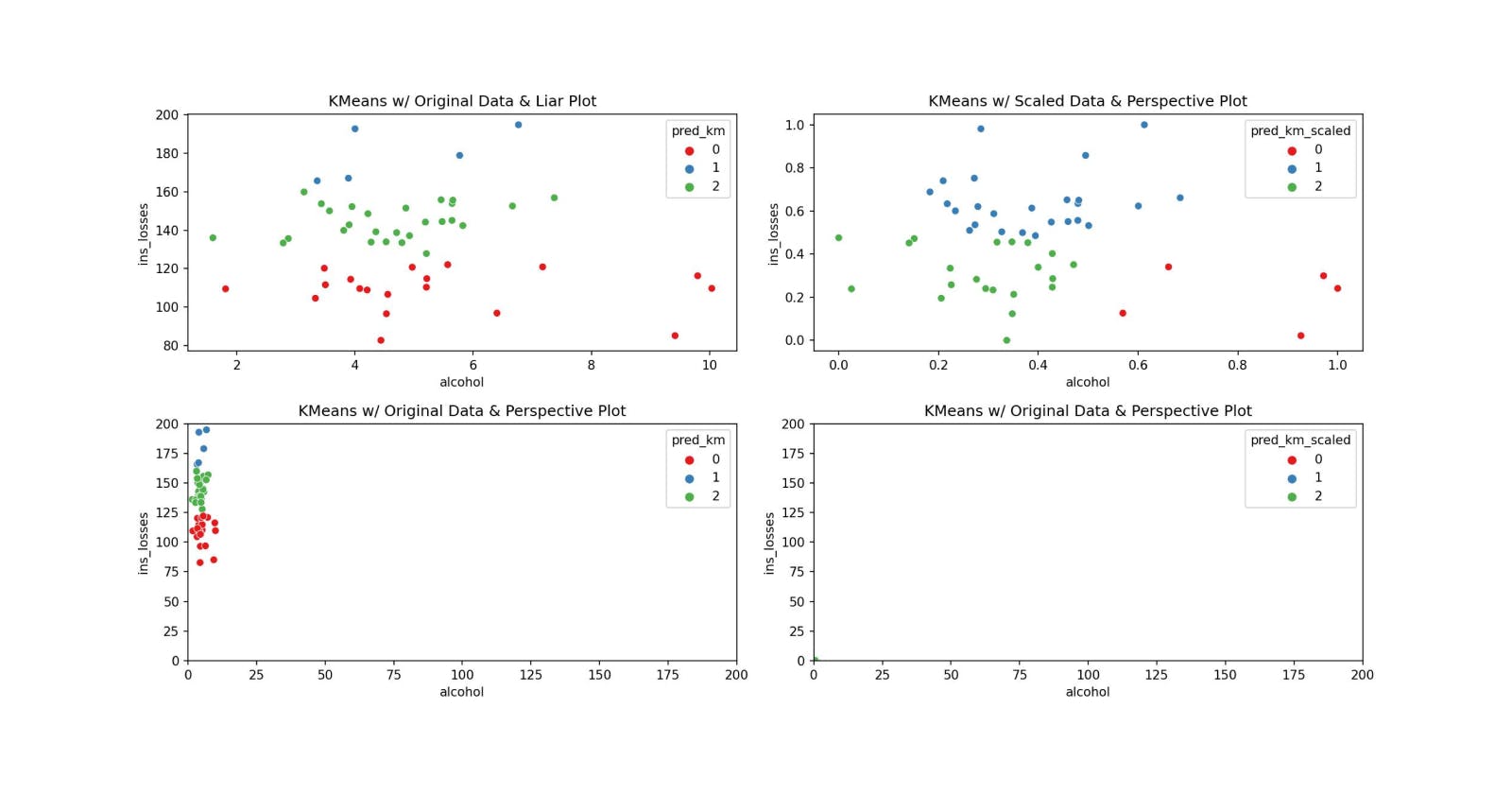
The following figure gives an overview of everything that has happened so far:

fig, ((ax1, ax2), (ax3, ax4)) = plt.subplots(2, 2, figsize=(14, 7))

sns.scatterplot(x='alcohol', y='ins_losses', hue='pred_km',
                data=df_pred, palette='Set1', ax=ax1);

sns.scatterplot(x='alcohol', y='ins_losses', hue=df_pred.pred_km_scaled,
                data=df_scaled, palette='Set1', ax=ax2);

sns.scatterplot(x='alcohol', y='ins_losses', hue='pred_km',
                data=df_pred, palette='Set1', ax=ax3);

sns.scatterplot(x='alcohol', y='ins_losses', hue=df_pred.pred_km_scaled,
                data=df_scaled, palette='Set1', ax=ax4);

ax3.set_xlim(0, 200)
ax3.set_ylim(0, 200)

ax4.set_xlim(0, 200)
ax4.set_ylim(0, 200)

ax1.set_title('KMeans w/ Original Data & Liar Plot')
ax2.set_title('KMeans w/ Scaled Data & Perspective Plot')
ax3.set_title('KMeans w/ Original Data & Perspective Plot')
ax4.set_title('KMeans w/ Original Data & Perspective Plot')

plt.tight_layout()

Other Clustering Models in Python

Visit the sklearn website to see how many different clustering methods are and how they differ from each other.

Let's pick two new models and compute them:

Agglomerative Clustering

We follow the same procedure as for any Machine Learning model from the Scikit-Learn library:

Fit the Model

from sklearn.cluster import AgglomerativeClustering

model_ac = AgglomerativeClustering(n_clusters=3)
model_ac.fit(df_scaled)

AgglomerativeClustering(n_clusters=3)

Calculate Predictions

model_ac.fit_predict(X=df_scaled)

array([0, 0, 1, 0, 0, 0, 0, 0, 0, 0, 0, 1, 1, 0, 1, 1, 0, 0, 0, 1, 0, 0, 0, 0, 0, 0, 2, 1, 0, 1, 0, 1, 0, 1, 2, 0, 0, 1, 0, 0, 2, 1, 0, 0, 0, 1, 0, 1, 0, 1, 1])

Create a New Column for the Predictions

df_pred['pred_ac'] = model_ac.fit_predict(X=df_scaled)
df_pred

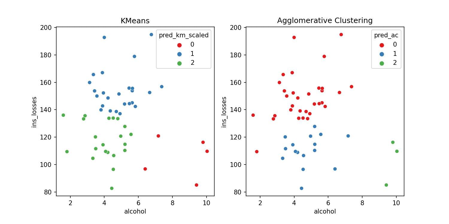
Visualize the Model

We can observe how the second group takes three points with the Agglomerative Clustering while the KMeans gather five points in the second group.

As they are different algorithms, they are expected to produce different results. If you'd like to understand which models you should use, you may know how the algorithm works. We don't explain it in this series because we want to make it simple.

fig, (ax1, ax2) = plt.subplots(1, 2, figsize=(10, 5))

sns.scatterplot(x='alcohol', y='ins_losses', hue='pred_km_scaled',
                data=df_pred, palette='Set1', ax=ax1);

sns.scatterplot(x='alcohol', y='ins_losses', hue='pred_ac',
                data=df_pred, palette='Set1', ax=ax2)

ax1.set_title('KMeans')
ax2.set_title('Agglomerative Clustering');

Spectral Clustering

We follow the same procedure as for any Machine Learning model from the Scikit-Learn library:

Fit the Model

from sklearn.cluster import SpectralClustering

model_sc = SpectralClustering(n_clusters=3)
model_sc.fit(df_scaled)

SpectralClustering(n_clusters=3)

Calculate Predictions

model_sc.fit_predict(X=df_scaled)

array([0, 2, 2, 0, 0, 2, 0, 0, 2, 0, 0, 1, 2, 0, 2, 2, 2, 0, 0, 2, 0, 2, 0, 2, 0, 0, 1, 2, 0, 2, 0, 2, 0, 2, 1, 2, 0, 2, 0, 0, 1, 1, 0, 0, 2, 2, 0, 2, 0, 2, 2], dtype=int32)

Create a New Column for the Predictions

df_pred['pred_sc'] = model_sc.fit_predict(X=df_scaled)
df_pred

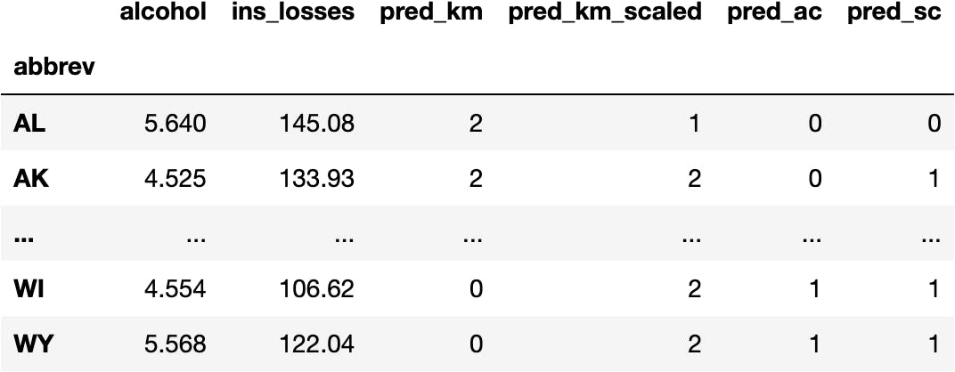
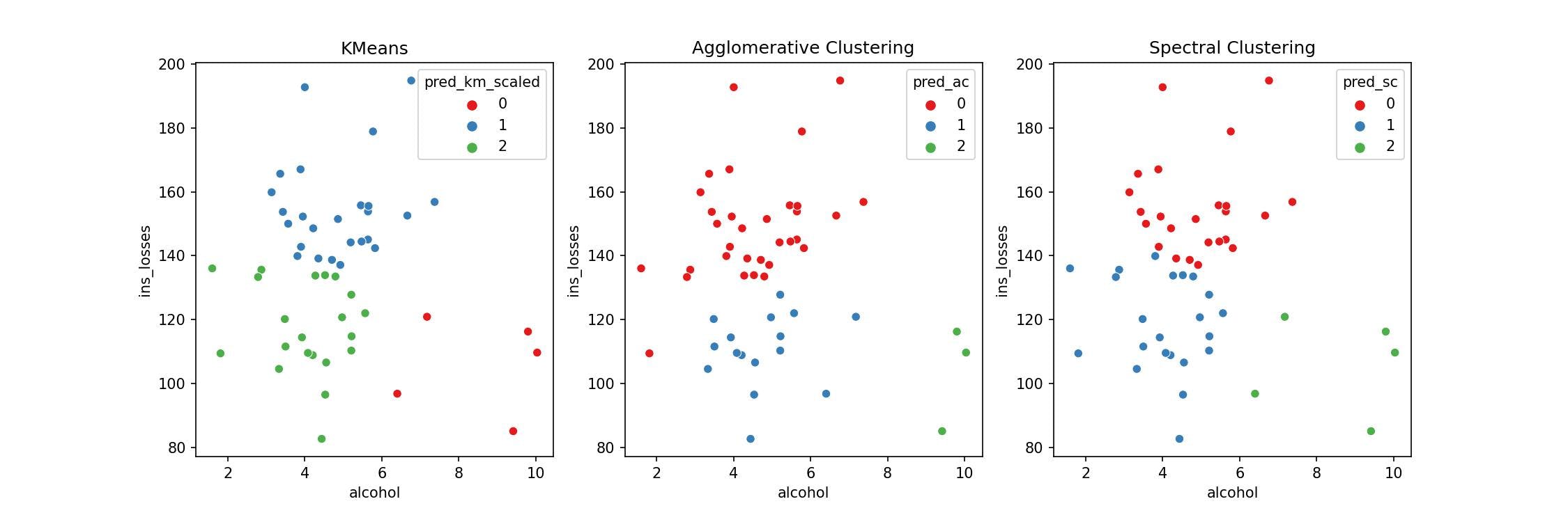
Visualize the Model

Let's visualize all models together and appreciate the minor differences because they cluster the groups differently.

fig, (ax1, ax2, ax3) = plt.subplots(1, 3, figsize=(15, 5))

ax1.set_title('KMeans')
sns.scatterplot(x='alcohol', y='ins_losses', hue='pred_km_scaled',
                data=df_pred, palette='Set1', ax=ax1);

ax2.set_title('Agglomerative Clustering')
sns.scatterplot(x='alcohol', y='ins_losses', hue='pred_ac',
                data=df_pred, palette='Set1', ax=ax2);

ax3.set_title('Spectral Clustering')
sns.scatterplot(x='alcohol', y='ins_losses', hue='pred_sc',
                data=df_pred, palette='Set1', ax=ax3);

Takeaway

Once again, you don't need to know the maths behind every Machine Learning model to build them. However, I hope you are getting a sense of the patterns behind the Scikit-Learn library with this series of tutorials.

Use Case Conclusion

Let's arbitrarily choose the Agglomerative Clustering as our model and get back to you being the President of the USA. How would you describe the groups?

1. Higher ins_losses and lower alcohol

2. Lower ins_losses and lower alcohol

3. Lower ins_losses and higher alcohol

sns.scatterplot(x='alcohol', y='ins_losses', hue='pred_ac', data=df_pred, palette='Set1');

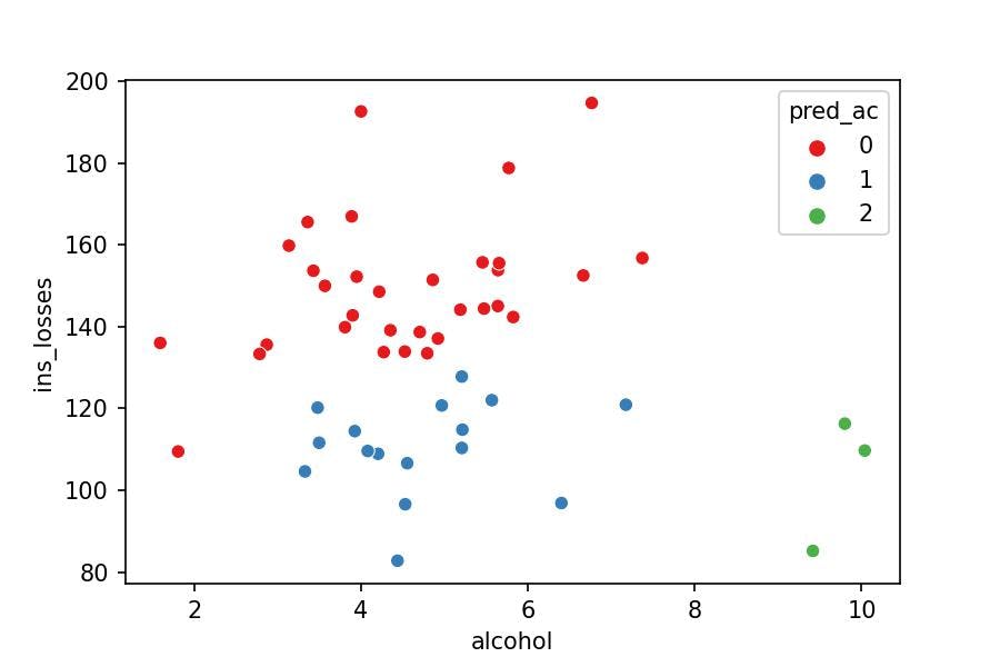
You would create different messages on the TV campaigns for the three groups separately and avoid deploying many more resources to develop fifty-one various TV campaigns (one for each State), which doesn't make sense because many of them are similar.