

#02 | The Decision Tree Classifier & Supervised Classification Models
This tutorial shows you the step-by-step resolution of possible errors you may get as you develop a Decision Tree Classifier.


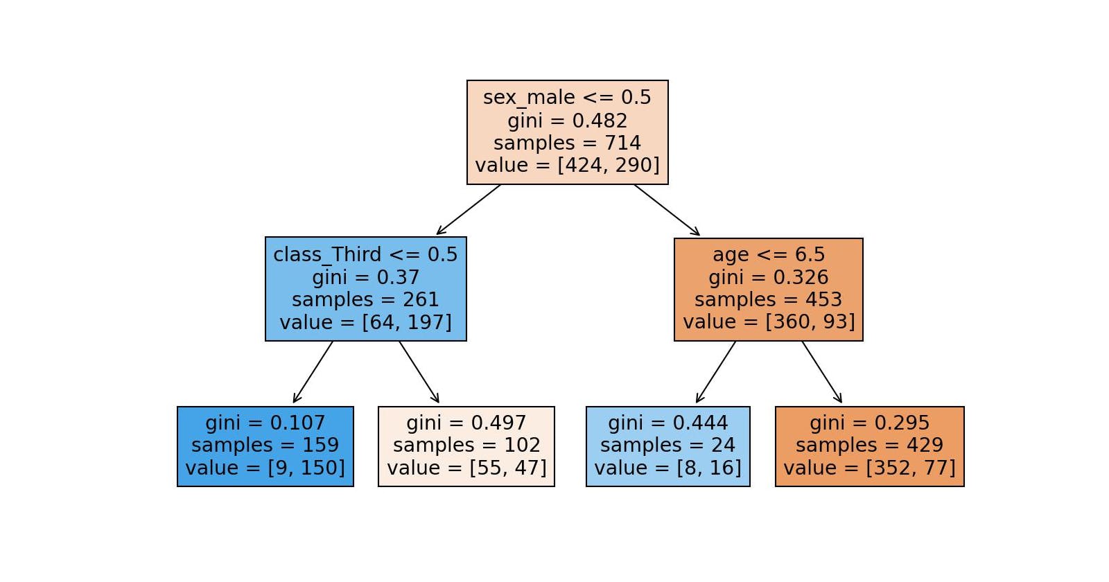
Table of contents
- Introduction to Supervised Classification Models
- Load the Data
- How do we compute a Decision Tree Model in Python?
- Data Preprocessing
- Other Classification Models
- Which One Is the Best Model? Why?
© Jesús López 2022
Don't miss out on his posts on LinkedIn to become a more efficient Python developer.
Introduction to Supervised Classification Models
Machine Learning is a field that focuses on getting a mathematical equation to make predictions. Although not all Machine Learning models work the same way.
Which types of Machine Learning models can we distinguish so far?
Classifiers to predict Categorical Variables
Regressors to predict Numerical Variables
The previous chapter covered the explanation of a Regressor model: Linear Regression.
This chapter covers the explanation of a Classification model: the Decision Tree.
Why do they belong to Machine Learning?
The Machine wants to get the best numbers of a mathematical equation such that the difference between reality and predictions is minimum:
Classifier evaluates the model based on prediction success rate y=?y^
Regressor evaluates the model based on the distance between real data and predictions (residuals) y−y^
There are many Machine Learning Models of each type.
You don't need to know the process behind each model because they all work the same way (see article). In the end, you will choose the one that makes better predictions.
This tutorial will show you how to develop a Decision Tree to calculate the probability of a person surviving the Titanic and the different evaluation metrics we can calculate on Classification Models.
Table of Important Content
🛀 How to preprocess/clean the data to fit a Machine Learning model?
Dummy Variables
Missing Data
🤩 How to visualize a Decision Tree model in Python step by step?
🤔 How to interpret the nodes and leaf's values of a Decision Tree plot?
⚠️ How to evaluate Classification models?
-
Sensitivity
Specificity
ROC Curve
🏁 How to compare Classification models to choose the best one?
Load the Data
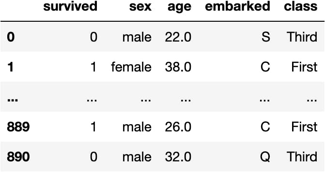
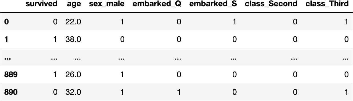
This dataset represents people (rows) aboard the Titanic
And their sociological characteristics (columns)
import seaborn as sns #!
import pandas as pd

df_titanic = sns.load_dataset(name='titanic')[['survived', 'sex', 'age', 'embarked', 'class']]
df_titanic
How do we compute a Decision Tree Model in Python?
We should know from the previous chapter that we need a function accessible from a Class in the library sklearn.
Import the Class
from sklearn.tree import DecisionTreeClassifier
Instantiante the Class
To create a copy of the original's code blueprint to not "modify" the source code.
model_dt = DecisionTreeClassifier()
Access the Function
The theoretical action we'd like to perform is the same as we executed in the previous chapter. Therefore, the function should be called the same way:
model_dt.fit()
---------------------------------------------------------------------------
TypeError Traceback (most recent call last)
/var/folders/24/tg28vxls25l9mjvqrnh0plc80000gn/T/ipykernel_3553/3699705032.py in ----> 1 model_dt.fit()
TypeError: fit() missing 2 required positional arguments: 'X' and 'y'
Why is it asking for two parameters: y and X?
y: target ~ independent ~ label ~ class variableX: explanatory ~ dependent ~ feature variables
Separate the Variables
target = df_titanic['survived']
explanatory = df_titanic.drop(columns='survived')
Fit the Model
model_dt.fit(X=explanatory, y=target)
---------------------------------------------------------------------------
ValueError: could not convert string to float: 'male'
Most of the time, the data isn't prepared to fit the model. So let's dig into why we got the previous error in the following sections.
Data Preprocessing
The error says:
ValueError: could not convert string to float: 'male'
From which we can interpret that the function .fit() does not accept values of string type like the ones in sex column:
df_titanic

Dummy Variables
Therefore, we need to convert the categorical columns to dummies (0s & 1s):
pd.get_dummies(df_titanic, drop_first=True)

df_titanic = pd.get_dummies(df_titanic, drop_first=True)
We separate the variables again to take into account the latest modification:
explanatory = df_titanic.drop(columns='survived')
target = df_titanic[['survived']]
Fit the Model Again
Now we should be able to fit the model:
model_dt.fit(X=explanatory, y=target)
---------------------------------------------------------------------------
ValueError: Input contains NaN, infinity or a value too large for dtype('float32').
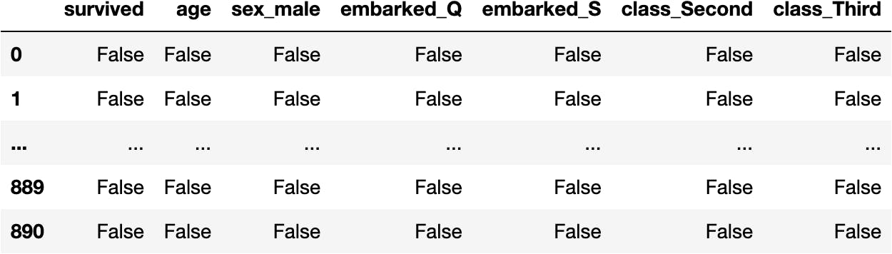
Missing Data
The data passed to the function contains missing data (NaN). Precisely 177 people from which we don't have the age:
df_titanic.isna()
df_titanic.isna().sum()
survived 0 age 177 sex_male 0 embarked_Q 0 embarked_S 0 class_Second 0 class_Third 0 dtype: int64
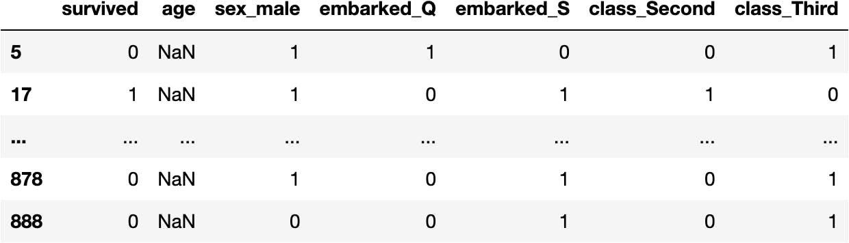
Who are the people who lack the information?
mask_na = df_titanic.isna().sum(axis=1) > 0
df_titanic[mask_na]
What could we do with them?
Drop the people (rows) who miss the age from the dataset.
Fill the age by the average age of other combinations (like males who survived)
Apply an algorithm to fill them.
We'll choose option 1 to simplify the tutorial.
Therefore, we go from 891 people:
df_titanic

To 714 people:
df_titanic.dropna()
df_titanic = df_titanic.dropna()
We separate the variables again to take into account the latest modification:
explanatory = df_titanic.drop(columns='survived')
target = df_titanic['survived']
Now we shouldn't have any more trouble with the data to fit the model.
Fit the Model Again
We don't get any errors because we correctly preprocess the data for the model.
Once the model is fitted, we may observe that the object contains more attributes because it has calculated the best numbers for the mathematical equation.
model_dt.fit(X=explanatory, y=target)
model_dt.__dict__
{'criterion': 'gini', 'splitter': 'best', 'max_depth': None, 'min_samples_split': 2, 'min_samples_leaf': 1, 'min_weight_fraction_leaf': 0.0, 'max_features': None, 'max_leaf_nodes': None, 'random_state': None, 'min_impurity_decrease': 0.0, 'class_weight': None, 'ccp_alpha': 0.0, 'feature_names_in_': array(['age', 'sex_male', 'embarked_Q', 'embarked_S', 'class_Second', 'class_Third'], dtype=object), 'n_features_in_': 6, 'n_outputs_': 1, 'classes_': array([0, 1]), 'n_classes_': 2, 'max_features_': 6, 'tree_': <sklearn.tree._tree.Tree at 0x16612cce0>}
Learn how to become an independent Machine Learning programmer who knows when to apply any ML algorithm to any dataset.
Predictions
Calculate Predictions
We have a fitted DecisionTreeClassifier. Therefore, we should be able to apply the mathematical equation to the original data to get the predictions:
model_dt.predict_proba(X=explanatory)[:5]
array([[0.82051282, 0.17948718], [0.05660377, 0.94339623], [0.53921569, 0.46078431], [0.05660377, 0.94339623], [0.82051282, 0.17948718]])
Add a New Column with the Predictions
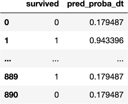
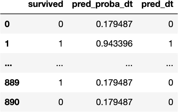
Let's create a new DataFrame to keep the information of the target and predictions to understand the topic better:
df_pred = df_titanic[['survived']].copy()
And add the predictions:
df_pred['pred_proba_dt'] = model_dt.predict_proba(X=explanatory)[:,1]
df_pred
How have we calculated those predictions?
Model Visualization
The Decision Tree model doesn't specifically have a mathematical equation. But instead, a set of conditions is represented in a tree:
from sklearn.tree import plot_tree

plot_tree(decision_tree=model_dt);
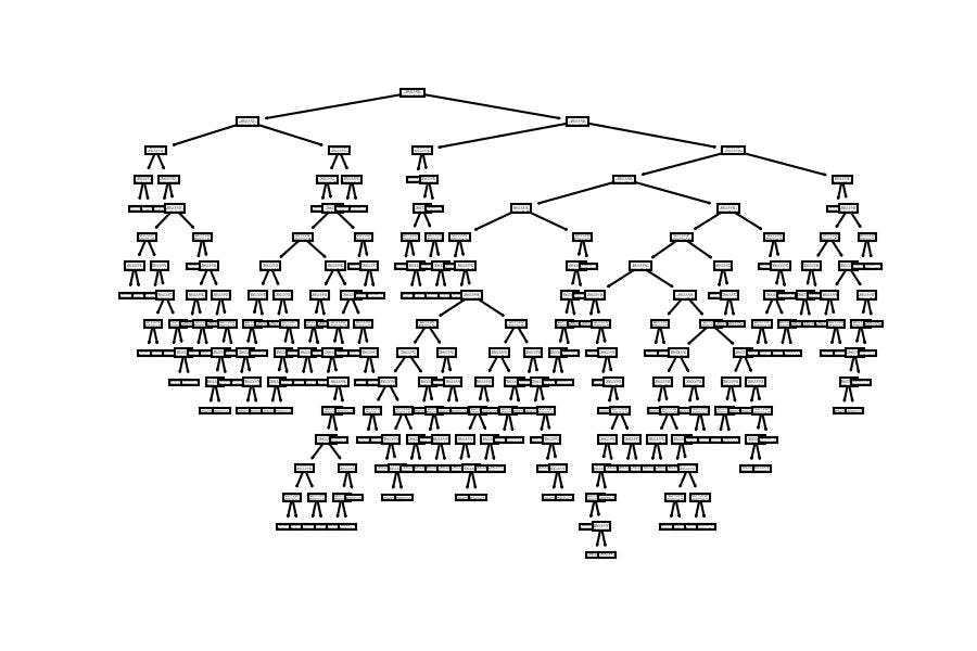
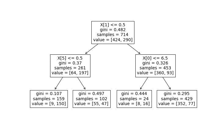
There are many conditions; let's recreate a shorter tree to explain the Mathematical Equation of the Decision Tree:
model_dt = DecisionTreeClassifier(max_depth=2)
model_dt.fit(X=explanatory, y=target)

plot_tree(decision_tree=model_dt);
Let's make the image bigger:
import matplotlib.pyplot as plt

plt.figure(figsize=(10,6))
plot_tree(decision_tree=model_dt);
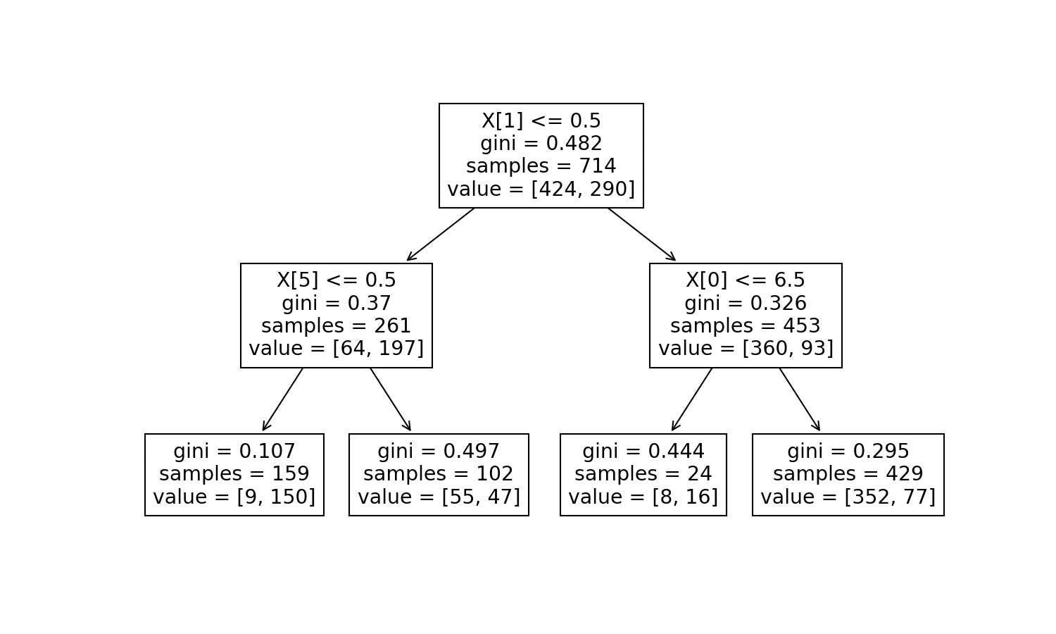
The conditions are X[2]<=0.5. The X[2] means the 3rd variable (Python starts counting at 0) of the explanatory ones. If we'd like to see the names of the columns, we need to add the feature_names parameter:
explanatory.columns
Index(['age', 'sex_male', 'embarked_Q', 'embarked_S', 'class_Second', 'class_Third'], dtype='object')
import matplotlib.pyplot as plt

plt.figure(figsize=(10,6))
plot_tree(decision_tree=model_dt, feature_names=explanatory.columns);
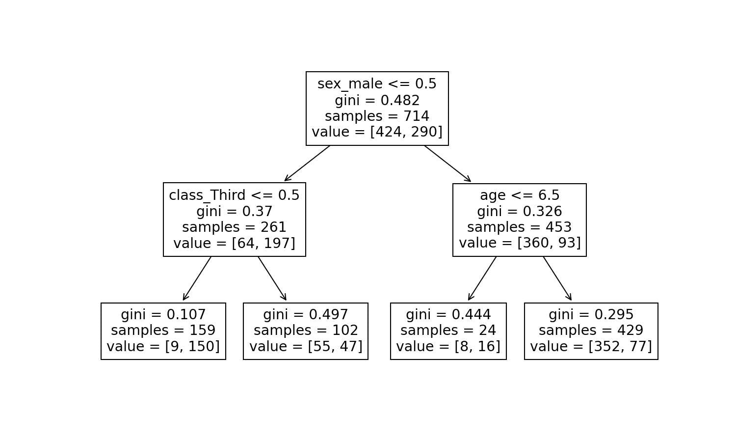
Let's add some colours to see how the predictions will go based on the fulfilled conditions:
import matplotlib.pyplot as plt

plt.figure(figsize=(10,6))
plot_tree(decision_tree=model_dt, feature_names=explanatory.columns, filled=True);
How does the Decision Tree Algorithm computes the Mathematical Equation?
The Decision Tree and the Linear Regression algorithms look for the best numbers in a mathematical equation. The following video explains how the Decision Tree configures the equation:
Model Interpretation
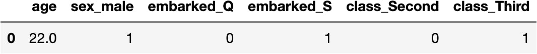
Let's take a person from the data to explain how the model makes a prediction. For storytelling, let's say the person's name is John.
John is a 22-year-old man who took the titanic on 3rd class but didn't survive:
df_titanic[:1]

To calculate the chances of survival in a person like John, we pass the explanatory variables of John:
explanatory[:1]
To the function .predict_proba() and get a probability of 17.94%:
model_dt.predict_proba(X=explanatory[:1])
array([[0.82051282, 0.17948718]])
But wait, how did we get to the probability of survival of 17.94%?
Let's explain it step-by-step with the Decision Tree visualization:
plt.figure(figsize=(10,6))
plot_tree(decision_tree=model_dt, feature_names=explanatory.columns, filled=True);

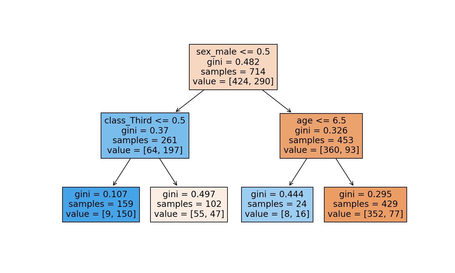
Based on the tree, the conditions are:
1st condition
- sex_male (John=1) <= 0.5 ~ False
John doesn't fulfil the condition; we move to the right side of the tree.
2nd condition
- age (John=22.0) <= 6.5 ~ False
John doesn't fulfil the condition; we move to the right side of the tree.
Leaf
The ultimate node, the leaf, tells us that the training dataset contained 429 males older than 6.5 years old.
Out of the 429, 77 survived, but 352 didn't make it.
Therefore, the chances of John surviving according to our model are 77 divided by 429:
77/429
0.1794871794871795
We get the same probability; John had a 17.94% chance of surviving the Titanic accident.
Model's Score
Calculate the Score
As always, we should have a function to calculate the goodness of the model:
model_dt.score(X=explanatory, y=target)
0.8025210084033614
The model can correctly predict 80.25% of the people in the dataset.
What's the reasoning behind the model's evaluation?
The Score Step-by-step
As we saw earlier, the classification model calculates the probability for an event to occur. The function .predict_proba() gives us two probabilities in the columns: people who didn't survive (0) and people who survived (1).
model_dt.predict_proba(X=explanatory)[:5]
array([[0.82051282, 0.17948718], [0.05660377, 0.94339623], [0.53921569, 0.46078431], [0.05660377, 0.94339623], [0.82051282, 0.17948718]])
We take the positive probabilities in the second column:
df_pred['pred_proba_dt'] = model_dt.predict_proba(X=explanatory)[:, 1]
At the time to compare reality (0s and 1s) with the predictions (probabilities), we need to turn probabilities higher than 0.5 into 1, and 0 otherwise.
import numpy as np

df_pred['pred_dt'] = np.where(df_pred.pred_proba_dt > 0.5, 1, 0)
df_pred
The simple idea of the accuracy is to get the success rate on the classification: how many people do we get right?
We compare if the reality is equal to the prediction:
comp = df_pred.survived == df_pred.pred_dt
comp
0 True 1 True ...
889 False 890 True Length: 714, dtype: bool
If we sum the boolean Series, Python will take True as 1 and 0 as False to compute the number of correct classifications:
comp.sum()
573
We get the score by dividing the successes by all possibilities (the total number of people):
comp.sum()/len(comp)
0.8025210084033614
It is also correct to do the mean on the comparisons because it's the sum divided by the total. Observe how you get the same number:
comp.mean()
0.8025210084033614
But it's more efficient to calculate this metric with the function .score():
model_dt.score(X=explanatory, y=target)
0.8025210084033614
The Confusion Matrix to Compute Other Classification Metrics
Can we think that our model is 80.25% of good and be happy with it?
- We should not because we might be interested in the accuracy of each class (survived or not) separately. But first, we need to compute the confusion matrix:
from sklearn.metrics import confusion_matrix, ConfusionMatrixDisplay

cm = confusion_matrix(
    y_true=df_pred.survived,
    y_pred=df_pred.pred_dt
)

CM = ConfusionMatrixDisplay(cm)
CM.plot();
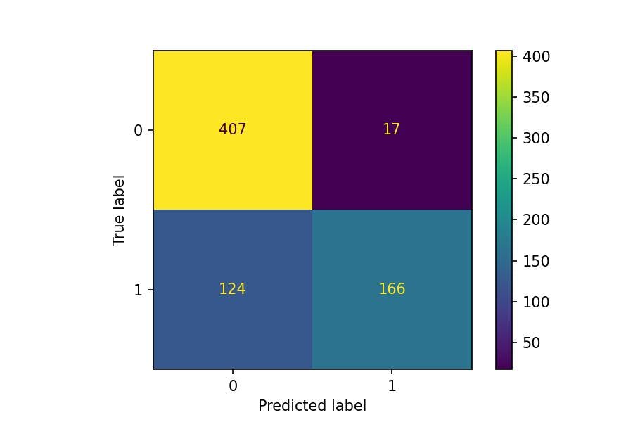
Looking at the first number of the confusion matrix, we have 407 people who didn't survive the Titanic in reality and the predictions.
It is not the case with the number 17. Our model classified 17 people as survivors when they didn't.
The success rate of the negative class, people who didn't survive, is called the specificity: $407/(407+17)$.
Whereas the success rate of the positive class, people who did survive, is called the sensitivity: $166/(166+124)$.
Specificity (Recall=0)
cm[0,0]
407
cm[0,:]
array([407, 17])
cm[0,0]/cm[0,:].sum()
0.9599056603773585
sensitivity = cm[0,0]/cm[0,:].sum()
Sensitivity (Recall=1)
cm[1,1]
166
cm[1,:]
array([124, 166])
cm[1,1]/cm[1,:].sum()
0.5724137931034483
sensitivity = cm[1,1]/cm[1,:].sum()
Classification Report
We could have gotten the same metrics using the function classification_report(). Look a the recall (column) of rows 0 and 1, specificity and sensitivity, respectively:
from sklearn.metrics import classification_report

report = classification_report(
    y_true=df_pred.survived,
    y_pred=df_pred.pred_dt
)

print(report)
precision recall f1-score support
0 0.77 0.96 0.85 424 1 0.91 0.57 0.70 290
accuracy 0.80 714 macro avg 0.84 0.77 0.78 714 weighted avg 0.82 0.80 0.79 714
We can also create a nice DataFrame to later use the data for simulations:
report = classification_report(
    y_true=df_pred.survived,
    y_pred=df_pred.pred_dt,
    output_dict=True
)

pd.DataFrame(report)
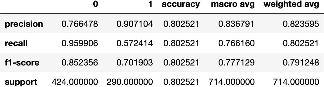
Our model is not as good as we thought if we predict the people who survived; we get 57.24% of survivors right.
How can we then assess a reasonable rate for our model?
ROC Curve
Watch the following video to understand how the Area Under the Curve (AUC) is a good metric because it sort of combines accuracy, specificity and sensitivity:
We compute this metric in Python as follows:
import matplotlib.pyplot as plt
import numpy as np
from sklearn import metrics

y = df_pred.survived
pred = model_dt.predict_proba(X=explanatory)[:,1]

fpr, tpr, thresholds = metrics.roc_curve(y, pred)
roc_auc = metrics.auc(fpr, tpr)

display = metrics.RocCurveDisplay(fpr=fpr, tpr=tpr, roc_auc=roc_auc,
                                  estimator_name='example estimator')
display.plot()
plt.show()
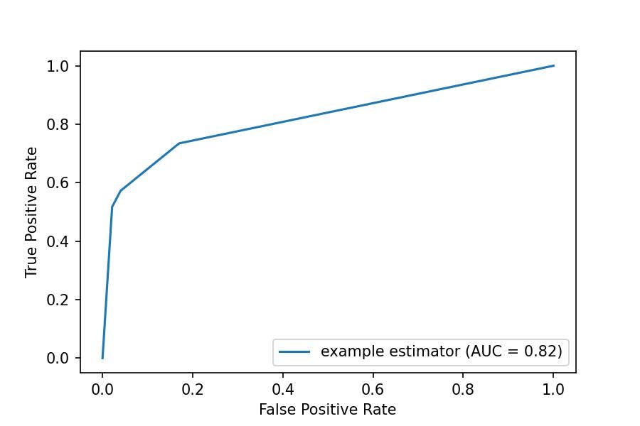
roc_auc
0.8205066688353937
Other Classification Models
Let's build other classification models by applying the same functions. In the end, computing Machine Learning models is the same thing all the time.
RandomForestClassifier() in Python
Fit the Model
from sklearn.ensemble import RandomForestClassifier

model_rf = RandomForestClassifier()
model_rf.fit(X=explanatory, y=target)
RandomForestClassifier()
Calculate Predictions
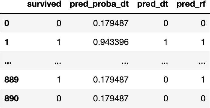
df_pred['pred_rf'] = model_rf.predict(X=explanatory)
df_pred
Model's Score
model_rf.score(X=explanatory, y=target)
0.9117647058823529
SVC() in Python
Fit the Model
from sklearn.svm import SVC

model_sv = SVC()
model_sv.fit(X=explanatory, y=target)
SVC()
Calculate Predictions
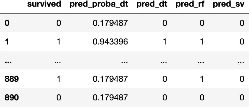
df_pred['pred_sv'] = model_sv.predict(X=explanatory)
df_pred
Model's Score
model_sv.score(X=explanatory, y=target)
0.6190476190476191
Which One Is the Best Model? Why?
To simplify the explanation, we use accuracy as the metric to compare the models. We have the Random Forest as the best model with an accuracy of 91.17%.
model_dt.score(X=explanatory, y=target)
0.8025210084033614
model_rf.score(X=explanatory, y=target)
0.9117647058823529
model_sv.score(X=explanatory, y=target)
0.6190476190476191
df_pred.head(10)


This work is licensed under a Creative Commons Attribution-NonCommercial-NoDerivatives 4.0 International License.