#01 | Getting Started with Pandas
A clear introduction to Pandas, a Python library to manipulate tabular data, where you can discover its many possibilities and get a concise overview.

I coach people to develop the Resolving Discipline that turns them into independent programmers.
Introduction
Programming is all about working with data.
We can work with many types of data structures. Nevertheless, the pandas DataFarme is the most useful because it contains functions that automate a lot of work by writing a simple line of code.
This tutorial will teach you how to work with the pandas.DataFrame object.
Before, we will demonstrate why working with simple Arrays (what most people do) makes your life more difficult than it should be.
The Array
An array is any object that can store more than one object. For example, the list:
[100, 134, 87, 99]
Let's say we are talking about the revenue our e-commerce has had over the last 4 months:
list_revenue = [100, 134, 87, 99]
We want to calculate the total revenue (i.e., we sum up the objects within the list):
list_revenue.sum()
---------------------------------------------------------------------------

AttributeError                            Traceback (most recent call last)

Input In [3], in <cell line: 1>()
----> 1 list_revenue.sum()


AttributeError: 'list' object has no attribute 'sum'
The list is a poor object which doesn't contain powerful functions.
What can we do then?
We convert the list to a powerful object such as the Series, which comes from pandas library.
import pandas

pandas.Series(list_revenue)
>>>
0    100
1    134
2     87
3     99
dtype: int64
series_revenue = pandas.Series(list_revenue)
Now we have a powerful object that can perform the .sum():
series_revenue.sum()
>>> 420
The Series
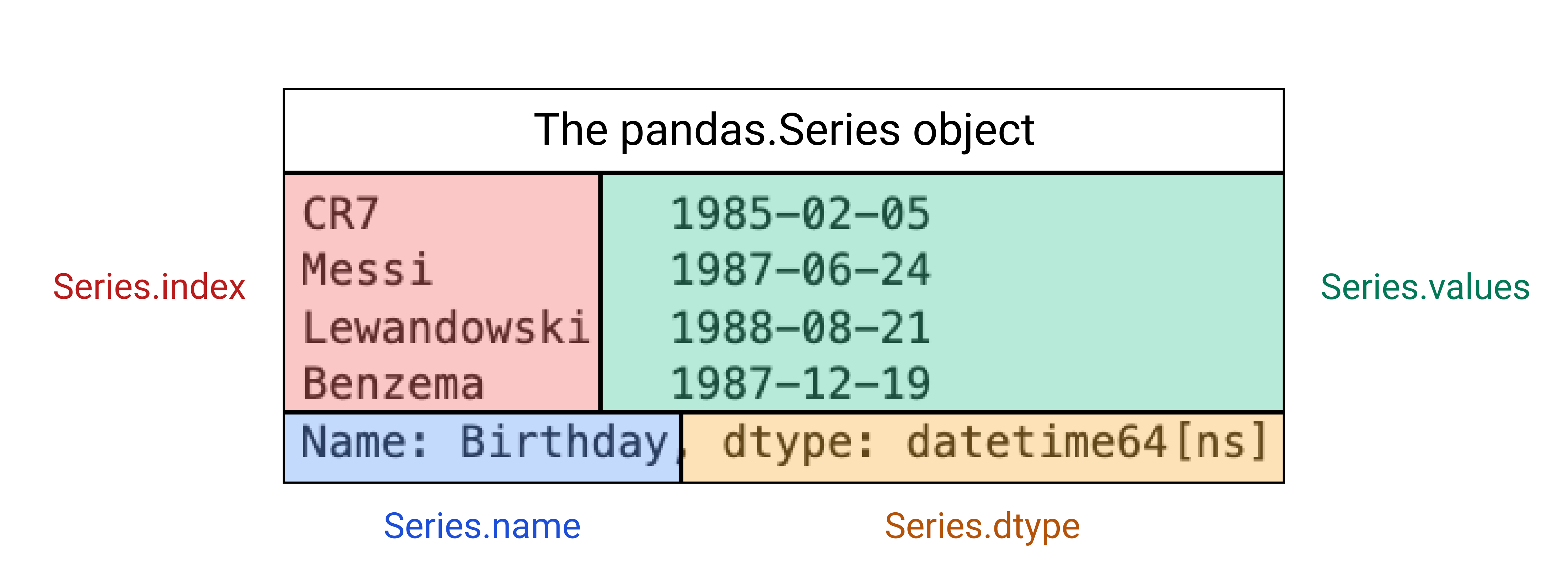
Within the Series, we can find more objects.
series_revenue
>>>
0    100
1    134
2     87
3     99
dtype: int64
The index
series_revenue.index
>>> RangeIndex(start=0, stop=4, step=1)
Let's change the elements of the index:
series_revenue.index = ['1st Month', '2nd Month', '3rd Month', '4th Month']
series_revenue
>>>
1st Month    100
2nd Month    134
3rd Month     87
4th Month     99
dtype: int64
The values
series_revenue.values
>>> array([100, 134, 87, 99])
The name
series_revenue.name
The Series doesn't contain a name. Let's define it:
series_revenue.name = 'Revenue'
series_revenue
>>>
1st Month    100
2nd Month    134
3rd Month     87
4th Month     99
Name: Revenue, dtype: int64
The dtype
The values of the Series (right-hand side) are determined by their data type (alias dtype):
series_revenue.dtype
>>> dtype('float64')
Let's change the values' dtype to be float (decimal numbers)
series_revenue.astype(float)
>>>
1st Month    100.0
2nd Month    134.0
3rd Month     87.0
4th Month     99.0
Name: Revenue, dtype: float64
series_revenue = series_revenue.astype(float)
Awesome Functions 😎
What else could we do with the Series object?
series_revenue.describe()
>>>
count      4.000000
mean     105.000000
std       20.215506
min       87.000000
25%       96.000000
50%       99.500000
75%      108.500000
max      134.000000
Name: Revenue, dtype: float64
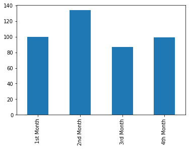
series_revenue.plot.bar();
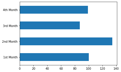
series_revenue.plot.barh();
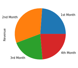
series_revenue.plot.pie();
The DataFrame
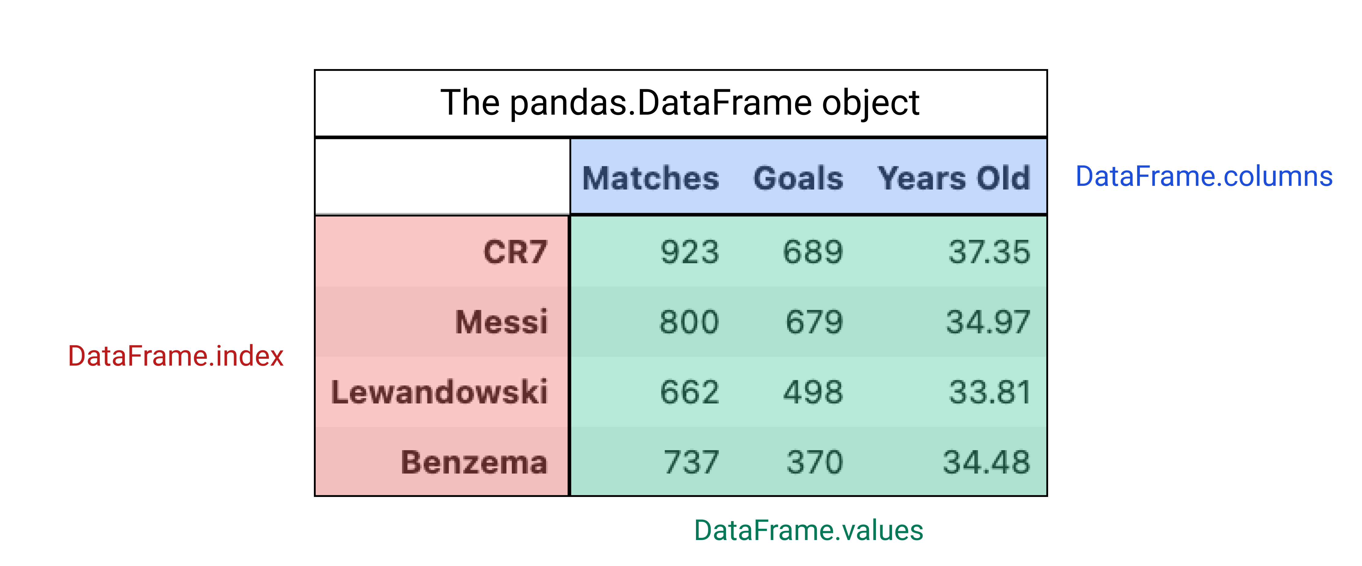
The DataFrame is a set of Series.
We will create another Series series_expenses to later put them together into a DataFrame.
pandas.Series(
    data=[20, 23, 21, 18],
    index=['1st Month','2nd Month','3rd Month','4th Month'],
    name='Expenses'
)
>>>
1st Month    20
2nd Month    23
3rd Month    21
4th Month    18
Name: Expenses, dtype: int64
series_expenses = pandas.Series(
    data=[20, 23, 21, 18],
    index=['1st Month','2nd Month','3rd Month','4th Month'],
    name='Expenses'
)
pandas.DataFrame(data=[series_revenue, series_expenses])
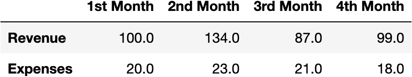
df_shop = pandas.DataFrame(data=[series_revenue, series_expenses])
Let's transpose the DataFrame to have the variables in columns:
df_shop.transpose()
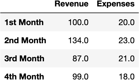
df_shop = df_shop.transpose()
The index
df_shop.index
>>> Index(['1st Month', '2nd Month', '3rd Month', '4th Month'], dtype='object')
The columns
df_shop.columns
>>> Index(['Revenue', 'Expenses'], dtype='object')
The values
df_shop.values
>>>
array([[100.,  20.],
       [134.,  23.],
       [ 87.,  21.],
       [ 99.,  18.]])
The shape
df_shop.shape
>>> (4, 2)
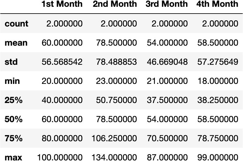
Awesome Functions 😎
What else could we do with the DataFrame object?
df_shop.describe()
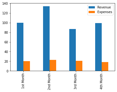
df_shop.plot.bar();
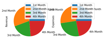
df_shop.plot.pie(subplots=True);
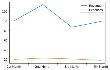
df_shop.plot.line();
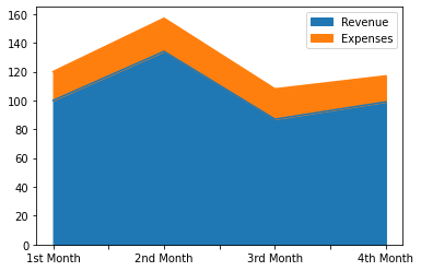
df_shop.plot.area();
We could also export the DataFrame to formatted data files:
df_shop.to_excel('data.xlsx')
df_shop.to_csv('data.csv')
Reading Data Tables from Files
JSON
Football Players
url = 'https://raw.githubusercontent.com/jsulopzs/data/main/football_players_stats.json'
pandas.read_json(url, orient='index')
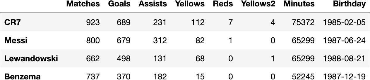
df_football = pandas.read_json(url, orient='index')
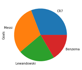
df_football.Goals.plot.pie();
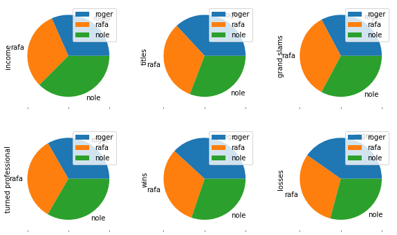
Tennis Players
url = 'https://raw.githubusercontent.com/jsulopzs/data/main/best_tennis_players_stats.json'
pandas.read_json(path_or_buf=url, orient='index')
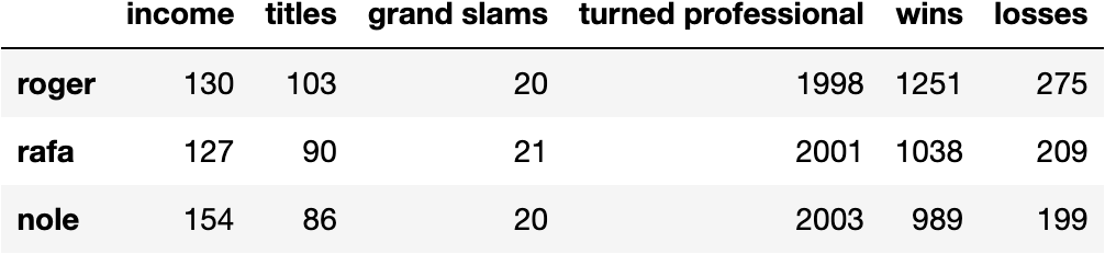
df_tennis = pandas.read_json(path_or_buf=url, orient='index')
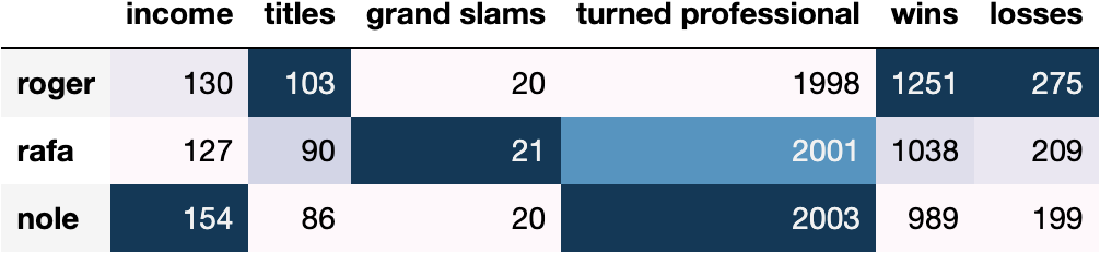
df_tennis.style.background_gradient()
df_tennis.plot.pie(subplots=True, layout=(2,3), figsize=(10,6));
HTML Web Page
pandas.read_html('https://www.skysports.com/la-liga-table/2021', index_col='Team')[0]
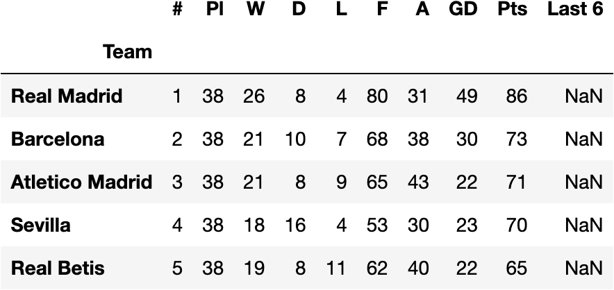
df_laliga = pandas.read_html('https://www.skysports.com/la-liga-table/2021', index_col='Team')[0]
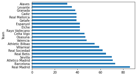
df_laliga.Pts.plot.barh();
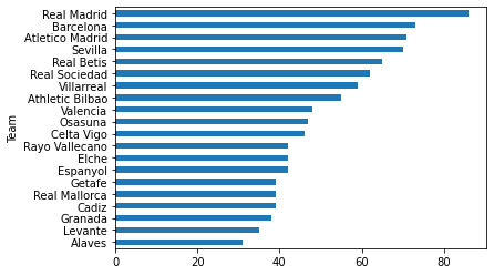
df_laliga.Pts.sort_values().plot.barh();
CSV
url = 'https://raw.githubusercontent.com/jsulopzs/data/main/internet_usage_spain.csv'
pandas.read_csv(filepath_or_buffer=url)
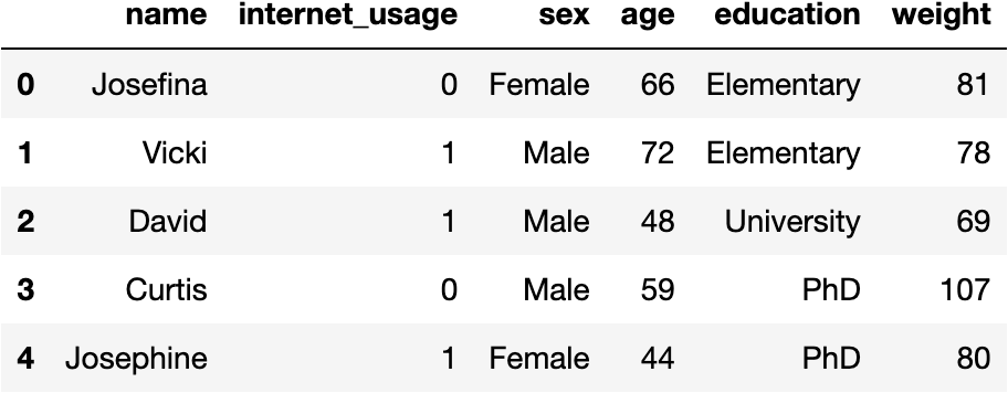
df_internet = pandas.read_csv(filepath_or_buffer=url)
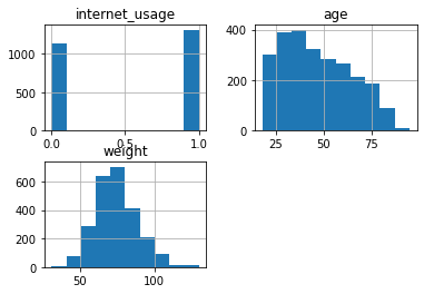
df_internet.hist();
df_internet.pivot_table(index='education', columns='internet_usage', aggfunc='size')
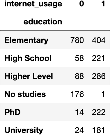
dfres = df_internet.pivot_table(index='education', columns='internet_usage', aggfunc='size')
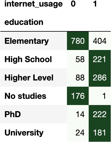
dfres.style.background_gradient('Greens', axis=1)

This work is licensed under a Creative Commons Attribution-NonCommercial-NoDerivatives 4.0 International License.