🎯 Chapter Importance

Machine Learning is all about calculating the best numbers of a mathematical equation.

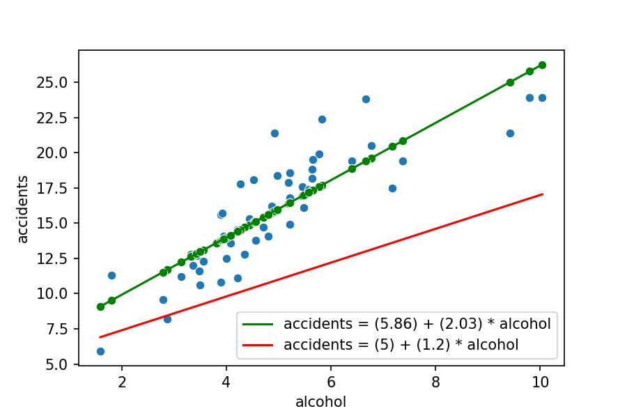
The form of a Linear Regression mathematical equation is as follows:

$$ y = (a) + (b) \cdot x $$

As we see in the following plot, not any mathematical equation is valid; the red line doesn't fit the real data (blue points), whereas the green one is the best.

How do we understand the development of Machine Learning models in Python to predict what may happen in the future?

This tutorial covers the topics described below using USA Car Crashes data to predict the accidents based on alcohol.

1. Step-by-step procedure to compute a Linear Regression:
   1. .fit() the numbers of the mathematical equation
   2. .predict() the future with the mathematical equation
   3. .score() how good is the mathematical equation
2. How to visualise the Linear Regression model?
3. How to evaluate Regression models step by step?
   • Residuals Sum of Squares
   • Total Sum of Squares
   • R Squared Ratio \(R^2\)
4. How to interpret the coefficients of the Linear Regression?
5. Compare the Linear Regression to other Machine Learning models such as:
   • Random Forest
   • Support Vector Machines
6. Why we don't need to know the maths behind every model to apply Machine Learning in Python?

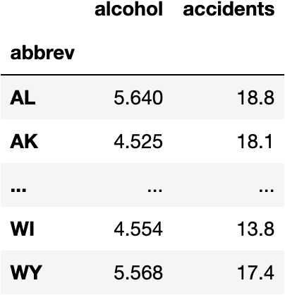
💽 Load the Data

• This dataset contains statistics about Car Accidents (columns)
• In each one of USA States (rows)

Visit this website if you want to know the measures of the columns.

import seaborn as sns #!

df_crashes = sns.load_dataset(name='car_crashes', index_col='abbrev')[['alcohol', 'total']]
df_crashes.rename({'total': 'accidents'}, axis=1, inplace=True)
df_crashes

🤖 How do we compute a Linear Regression Model in Python?

• As always, we need to use a function

Where is the function?

• It should be in a library

Which is the Python library for Machine Learning?

• Sci-Kit Learn, see website

Import the Class

How can we access the function to compute a Linear Regression model?

• We need to import the LinearRegression class within linear_model module:

from sklearn.linear_model import LinearRegression

Instantiante the Class

• Now, we create an instance model_lr of the class LinearRegression:

model_lr = LinearRegression()

Fit the Model

Which function applies the Linear Regression algorithm in which the Residual Sum of Squares is minimised?

model_lr.fit()

---

TypeError Traceback (most recent call last)

Input In [186], in () ----> 1 model_lr.fit()

TypeError: fit() missing 2 required positional arguments: 'X' and 'y'

Why is it asking for two parameters: y and X?

The algorithm must distinguish between the variable we want to predict (y), and the variables used to explain (X) the prediction.

• y: target ~ independent ~ label ~ class variable
• X: features ~ dependent ~ explanatory variables

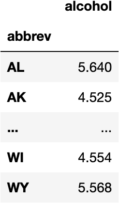
Separate the Variables

target = df_crashes['accidents']
features = df_crashes[['alcohol']]

Fit the Model Again

model_lr.fit(X=features, y=target)

LinearRegression()

Predictions

Calculate the Predictions

Take the historical data:

features

To calculate predictions through the Model's Mathematical Equation:

model_lr.predict(X=features)

array([17.32111171, 15.05486718, 16.44306899, 17.69509287, 12.68699734, 13.59756016, 13.76016066, 15.73575679, 9.0955587 , 16.40851638, 13.78455074, 20.44100889, 14.87600663, 14.70324359, 14.40446516, 13.8353634 , 14.54064309, 15.86177218, 19.6076813 , 15.06502971, 13.98780137, 11.69106925, 13.88211104, 11.5162737 , 16.94713055, 16.98371566, 24.99585551, 16.45729653, 15.41868581, 12.93089809, 12.23171592, 15.95526747, 13.10772614, 16.44306899, 26.26007443, 15.60161138, 17.58737003, 12.62195713, 17.32517672, 14.43088774, 25.77430543, 18.86988151, 17.3515993 , 20.84141263, 9.53254755, 14.15040187, 12.82724027, 12.96748321, 19.40239816, 15.11380986, 17.17477126])

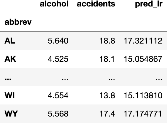
Add a New Column with the Predictions

Can you see the difference between reality and prediction?

• Model predictions aren't perfect; they don't predict the real data exactly. Nevertheless, they make a fair approximation allowing decision-makers to understand the future better.

df_crashes['pred_lr'] = model_lr.predict(X=features)
df_crashes

Model Visualization

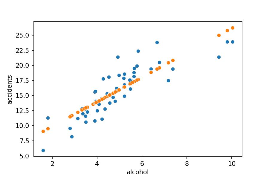
The orange dots reference the predictions lined up in a line because the Linear Regression model calculates the best coefficients (numbers) for a line's mathematical equation based on historical data.

import matplotlib.pyplot as plt

sns.scatterplot(x='alcohol', y='accidents', data=df_crashes)
sns.scatterplot(x='alcohol', y='pred_lr', data=df_crashes);

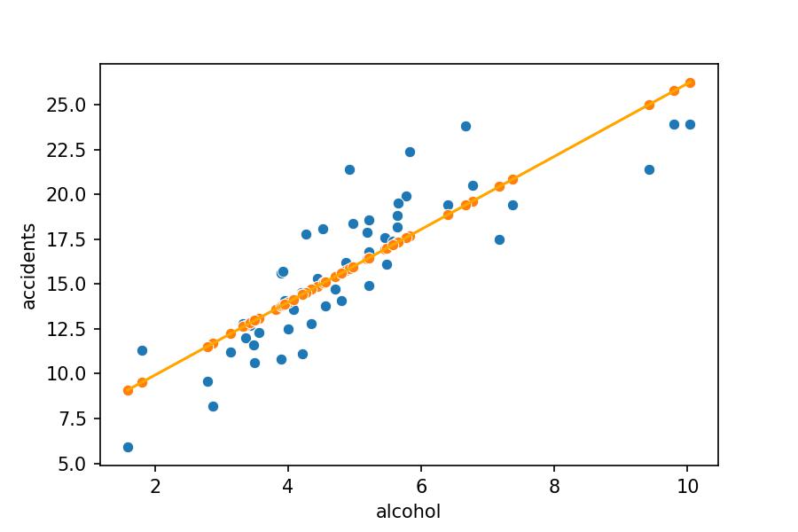
We have orange dots for the alcohol represented in our DataFrame. Were we to make estimations about all possible alcohol numbers, we'd get a sequence of consecutive points, which represented a line. Let's draw it with .lineplot() function:

sns.scatterplot(x='alcohol', y='accidents', data=df_crashes)
sns.scatterplot(x='alcohol', y='pred_lr', data=df_crashes);
sns.lineplot(x='alcohol', y='pred_lr', data=df_crashes, color='orange');

Model's Score

Calculate the Score

To measure the quality of the model, we use the .score() function to correctly calculate the difference between the model's predictions and reality.

model_lr.score(X=features, y=target)

0.7269492966665405

Explain the Score

Residuals

The step-by-step procedure of the previous calculation starts with the difference between reality and predictions:

df_crashes['accidents'] - df_crashes['pred_lr']

abbrev AL 1.478888 AK 3.045133 ...
WI -1.313810 WY 0.225229 Length: 51, dtype: float64

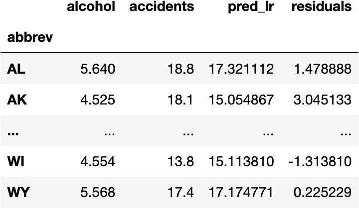
This difference is usually called residuals:

df_crashes['residuals'] = df_crashes['accidents'] - df_crashes['pred_lr']
df_crashes

We cannot use all the residuals to tell how good our model is. Therefore, we need to add them up:

df_crashes.residuals.sum()

1.4033219031261979e-13

Let's round to two decimal points to suppress the scientific notation:

df_crashes.residuals.sum().round(2)

0.0

But we get ZERO. Why?

The residuals contain positive and negative numbers; some points are above the line, and others are below the line.

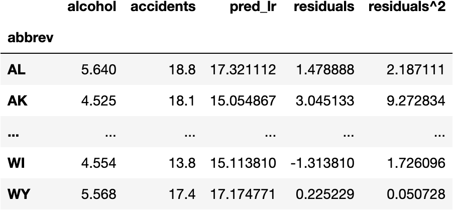
To turn negative values into positive values, we square the residuals:

df_crashes['residuals^2'] = df_crashes.residuals**2
df_crashes

And finally, add the residuals up to calculate the Residual Sum of Squares (RSS):

df_crashes['residuals^2'].sum()

231.96888653310063

RSS = df_crashes['residuals^2'].sum()

$$ RSS = \sum(y_i - \hat{y})^2 $$

where

• y_i is the real number of accidents
• $\hat y$ is the predicted number of accidents
• RSS: Residual Sum of Squares

Target's Variation

The model was made to predict the number of accidents.

We should ask: how good are the variation of the model's predictions compared to the variation of the real data (real number of accidents)?

We have already calculated the variation of the model's prediction. Now we calculate the variation of the real data by comparing each accident value to the average:

df_crashes.accidents

abbrev AL 18.8 AK 18.1 ... WI 13.8 WY 17.4 Name: accidents, Length: 51, dtype: float64

df_crashes.accidents.mean()

15.79019607843137

$$ y_i - \bar y $$

Where x is the number of accidents

df_crashes.accidents - df_crashes.accidents.mean()

abbrev AL 3.009804 AK 2.309804 ...
WI -1.990196 WY 1.609804 Name: accidents, Length: 51, dtype: float64

df_crashes['real_residuals'] = df_crashes.accidents - df_crashes.accidents.mean()
df_crashes

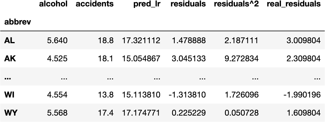
We square the residuals due for the same reason as before (convert negative values into positive ones):

df_crashes['real_residuals^2'] = df_crashes.real_residuals**2

$$ TTS = \sum(y_i - \bar y)^2 $$

where

• y_i is the number of accidents
• $\bar y$ is the average number of accidents
• TTS: Total Sum of Squares

And we add up the values to get the Total Sum of Squares (TSS):

df_crashes['real_residuals^2'].sum()

849.5450980392156

TSS = df_crashes['real_residuals^2'].sum()

The Ratio

The ratio between RSS and TSS represents how much our model fails concerning the variation of the real data.

RSS/TSS

0.2730507033334595

0.27 is the badness of the model as RSS represents the residuals (errors) of the model.

To calculate the goodness of the model, we need to subtract the ratio RSS/TSS to 1:

$$ R^2 = 1 - \frac{RSS}{TSS} = 1 - \frac{\sum(y_i - \hat{y})^2}{\sum(y_i - \bar y)^2} $$

1 - RSS/TSS

0.7269492966665405

The model can explain 72.69% of the total number of accidents variability.

The following image describes how we calculate the goodness of the model.

Model Interpretation

How do we get the numbers of the mathematical equation of the Linear Regression?

• We need to look inside the object model_lr and show the attributes with .__dict__ (the numbers were computed with the .fit() function):

model_lr.__dict__

{'fit_intercept': True, 'normalize': 'deprecated', 'copy_X': True, 'n_jobs': None, 'positive': False, 'feature_namesin': array(['alcohol'], dtype=object), 'n_featuresin': 1, 'coef_': array([2.0325063]), 'residues': 231.9688865331006, 'rank': 1, 'singular': array([12.22681605]), 'intercept': 5.857776154826299}

• intercept_ is the (a) number of the mathematical equation
• coef_ is the (b) number of the mathematical equation

$$ accidents = (a) + (b) \cdot alcohol \ accidents = (intercept_) + (coef_) \cdot alcohol \ accidents = (5.857) + (2.032) \cdot alcohol $$

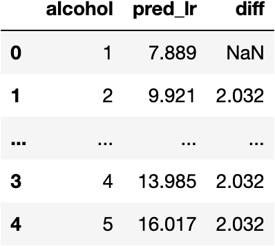
For every unit of alcohol increased, the number of accidents will increase by 2.032 units.

import pandas as pd

df_to_pred = pd.DataFrame({'alcohol': [1,2,3,4,5]})
df_to_pred['pred_lr'] = 5.857 + 2.032 * df_to_pred.alcohol
df_to_pred['diff'] = df_to_pred.pred_lr.diff()
df_to_pred

🚀 Other Regression Models

Could we make a better model that improves the current Linear Regression Score?

model_lr.score(X=features, y=target)

0.7269492966665405

• Let's try a Random Forest and a Support Vector Machines.

Do we need to know the maths behind these models to implement them in Python?

• No. As we explain in this tutorial, all you need to do is:

  1. fit()
  2. .predict()
  3. .score()
  4. Repeat

RandomForestRegressor() in Python

Fit the Model

from sklearn.ensemble import RandomForestRegressor

model_rf = RandomForestRegressor()
model_rf.fit(X=features, y=target)

RandomForestRegressor()

Calculate Predictions

model_rf.predict(X=features)

array([18.644 , 16.831 , 17.54634286, 21.512 , 12.182 , 13.15 , 12.391 , 17.439 , 7.775 , 17.74664286, 14.407 , 18.365 , 15.101 , 14.132 , 13.553 , 15.097 , 15.949 , 19.857 , 21.114 , 15.53 , 13.241 , 8.98 , 14.363 , 9.54 , 17.208 , 16.593 , 22.087 , 16.24144286, 14.478 , 11.51 , 11.59 , 18.537 , 11.77 , 17.54634286, 23.487 , 14.907 , 20.462 , 12.59 , 18.38 , 12.449 , 23.487 , 20.311 , 19.004 , 19.22 , 9.719 , 13.476 , 12.333 , 11.08 , 22.368 , 14.67 , 17.966 ])

df_crashes['pred_rf'] = model_rf.predict(X=features)

Model's Score

model_rf.score(X=features, y=target)

0.9549469198566546

Let's create a dictionary that stores the Score of each model:

dic_scores = {}
dic_scores['lr'] = model_lr.score(X=features, y=target)
dic_scores['rf'] = model_rf.score(X=features, y=target)

SVR() in Python

Fit the Model

from sklearn.svm import SVR

model_sv = SVR()
model_sv.fit(X=features, y=target)

SVR()

Calculate Predictions

model_sv.predict(X=features)

array([18.29570777, 15.18462721, 17.2224187 , 18.6633175 , 12.12434781, 13.10691581, 13.31612684, 16.21131216, 12.66062465, 17.17537208, 13.34820949, 19.38920329, 14.91415215, 14.65467023, 14.2131504 , 13.41560202, 14.41299448, 16.39752499, 19.4896662 , 15.20002787, 13.62200798, 11.5390483 , 13.47824339, 11.49818909, 17.87053595, 17.9144274 , 19.60736085, 17.24170425, 15.73585463, 12.35136579, 11.784815 , 16.53431108, 12.53373232, 17.2224187 , 19.4773929 , 16.01115736, 18.56379706, 12.06891287, 18.30002795, 14.25171609, 19.59597679, 19.37950461, 18.32794218, 19.29994413, 12.26345665, 13.84847453, 12.25128025, 12.38791686, 19.48212198, 15.27397732, 18.1357253 ])

df_crashes['pred_sv'] = model_sv.predict(X=features)

Model's Score

model_sv.score(X=features, y=target)

0.7083438012012769

dic_scores['sv'] = model_sv.score(X=features, y=target)

💪 Which One Is the Best? Why?

The best model is the Random Forest with a Score of 0.95:

pd.Series(dic_scores).sort_values(ascending=False)

rf 0.954947 lr 0.726949 sv 0.708344 dtype: float64

📊 Visualise the 3 Models

Let's put the following data:

df_crashes[['accidents', 'pred_lr', 'pred_rf', 'pred_sv']]

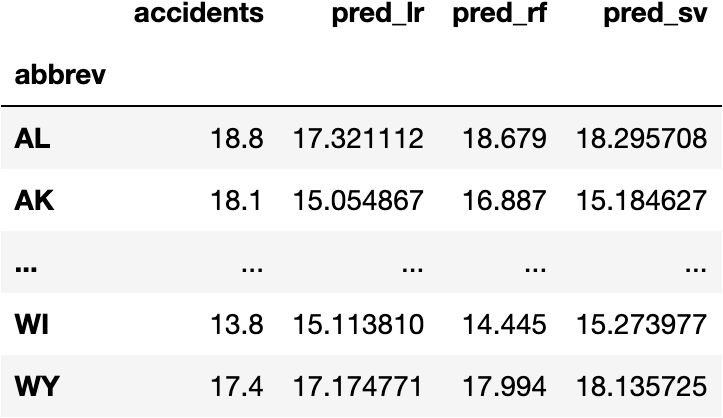
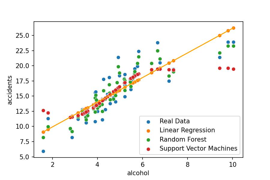
Into a plot:

sns.scatterplot(x='alcohol', y='accidents', data=df_crashes, label='Real Data')
sns.scatterplot(x='alcohol', y='pred_lr', data=df_crashes, label='Linear Regression')
sns.lineplot(x='alcohol', y='pred_lr', data=df_crashes, color='orange')
sns.scatterplot(x='alcohol', y='pred_rf', data=df_crashes, label='Random Forest')
sns.scatterplot(x='alcohol', y='pred_sv', data=df_crashes, label='Support Vector Machines');

This work is licensed under a Creative Commons Attribution-NonCommercial-NoDerivatives 4.0 International License.