#03 | Grouping & Pivot Tables
Learn how to summarise the information using the pandas DataFrame in order to become an efficient Data Analyst
© Jesús López 2022
Ask him any doubt on Twitter or LinkedIn
Possibilities
Look at the following example as an aspiration you can achieve if you fully understand and replicate this whole tutorial with your data.
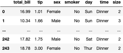
Let's load a dataset that contains information from transactions in tables (rows) at a restaurant considering socio-demographic and economic variables (columns).
import seaborn as sns

df_tips = sns.load_dataset('tips')
df_tips
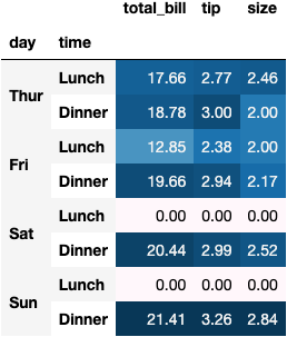
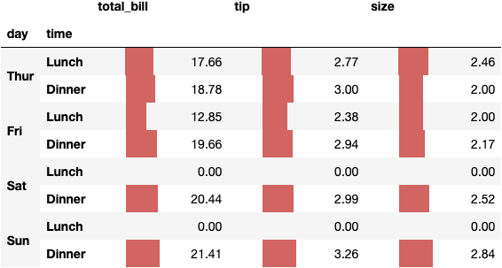
Grouping data to summarise the information helps you identify conclusions. For example, the summary below shows that Dinners on Sundays come to the best customers because they:
Spend more on average ($21.41)
Give more tips on average ($3.25)
Come more people at the same table on average ($2.84)
df_tips.groupby(by=['day', 'time'])\
    .mean()\
    .fillna(0)\
    .style.format('{:.2f}').background_gradient(axis=0)
df_tips.groupby(by=['day', 'time'])\
    .mean()\
    .fillna(0)\
    .style.format('{:.2f}').bar(axis=0, width=50, align='zero')
Let's dig into the details of the .groupby() function from the basics in the following sections.
Grouping by 1 Column
We use the .groupby() function to generate an object that contains as many DataFrames as categories are in the column.
df_tips.groupby('sex')
As we have two groups in sex (Female and Male), the length of the DataFrameGroupBy object returned by the groupby() function is 2:
len(df_tips.groupby('sex'))
How can we work with the object DataFrameGroupBy?
Calculate the Average for All Columns
We use the .mean() function to get the average of the numerical columns for the two groups:
df_tips.groupby('sex').mean()
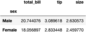
A pretty and simple syntax to summarise the information, right?
- But what's going on inside the
DataFrameGroupByobject?
df_tips.groupby('sex')
df_grouped = df_tips.groupby('sex')
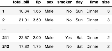
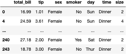
The DataFrameGroupBy object contains 2 DataFrames. To see one of them DataFrame you need to use the function .get_group() and pass the group whose DataFrame you'd like to return:
df_grouped.get_group('Male')
df_grouped.get_group('Female')
Learn how to become an independent Data Analyist programmer who knows how to extract meaningful insights from Data Visualizations.
As the DataFrameGroupBy distinguish the categories, at the moment we apply an aggregation function (click here to see a list of them), we will get the mathematical operations for those groups separately:
df_grouped.mean()
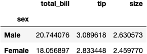
We could apply the function to each DataFrame separately. Although it is not the point of the .groupby() function.
df_grouped.get_group('Male').mean(numeric_only=True)
df_grouped.get_group('Female').mean(numeric_only=True)
Compute Functions to 1 Column
To get the results for just 1 column of interest, we access the column:
df_grouped.total_bill
And use the aggregation function we wish, .sum() in this case:
df_grouped.total_bill.sum()
We get the result for just 1 column (total_bill) because the DataFrames generated at .groupby() are accessed as if they were simple DataFrames:
df_grouped.get_group('Female')
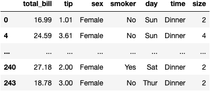
df_grouped.get_group('Female').total_bill
df_grouped.get_group('Female').total_bill.sum()
df_grouped.get_group('Male').total_bill.sum()
df_grouped.total_bill.sum()
Grouping by 2 Columns
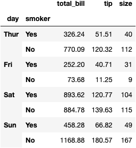
So far, we have summarised the data based on the categories of just one column. But, what if we'd like to summarise the data based on the combinations of the categories within different categorical columns?
Compute 1 Function
df_tips.groupby(by=['day', 'smoker']).sum()
Pivot Tables
We could have also used another function .pivot_table() to get the same numbers:
df_tips.pivot_table(index='day', columns='smoker', aggfunc='sum')
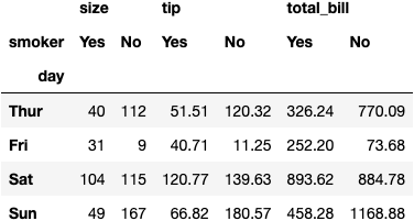
Which one is best?
- I leave it up to your choice; I'd prefer to use the
.pivot_table()because the syntax makes it more accessible.
Compute More than 1 Function
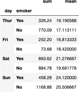
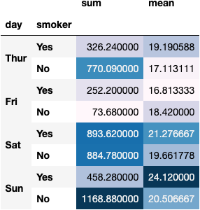
The thing doesn't stop here; we can even compute different aggregation functions at the same time:
Groupby
df_tips.groupby(by=['day', 'smoker'])\
    .total_bill\
    .agg(func=['sum', 'mean'])
Pivot Table
df_tips.pivot_table(index='day', columns='smoker',
                    values='total_bill', aggfunc=['sum', 'mean'])
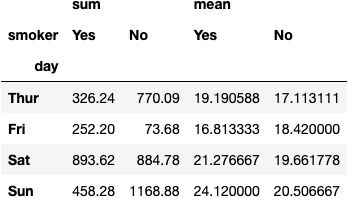
dfres = df_tips.pivot_table(index='day', columns='smoker',
                    values='total_bill', aggfunc=['sum', 'mean'])
You could even style the output DataFrame:
dfres.style.background_gradient()
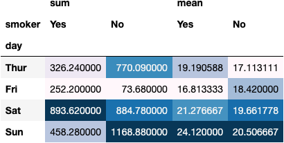
For me, it's nicer than styling the .groupby() returned DataFrame.
As we say in Spain:
Pa' gustos los colores!
df_tips.groupby(by=['day', 'smoker']).total_bill.agg(func=['sum', 'mean'])
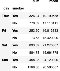
dfres = df_tips.groupby(by=['day', 'smoker']).total_bill.agg(func=['sum', 'mean'])
dfres.style.background_gradient()
Pivot Tables in Depth
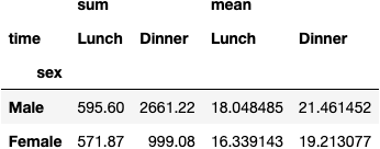
We can compute more than one mathematical operation:
df_tips.pivot_table(index='sex', columns='time',
                    aggfunc=['sum', 'mean'], values='total_bill')
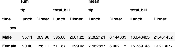
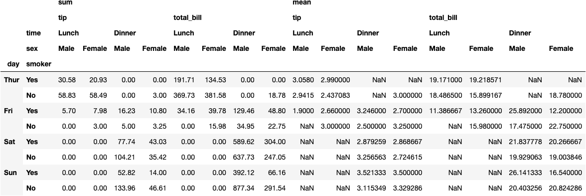
And use more than one column in each of the parameters:
df_tips.pivot_table(index='sex', columns='time',
                    aggfunc=['sum', 'mean'], values=['total_bill', 'tip'])
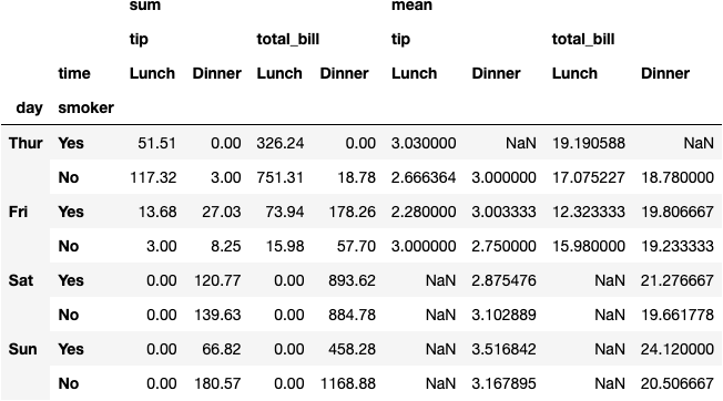
df_tips.pivot_table(index=['day', 'smoker'], columns='time',
                    aggfunc=['sum', 'mean'], values=['total_bill', 'tip'])
df_tips.pivot_table(index=['day', 'smoker'], columns=['time', 'sex'],
                    aggfunc=['sum', 'mean'], values=['total_bill', 'tip'])
The .size() Function
.groupby()
1 Variable to Group By
The .size() is a function used to count the number of rows (observations) in each of the DataFrames generated by .groupby().
df_grouped.size()
2 Variables to Group By
df_tips.groupby(by=['sex', 'time']).size()
.pivot_table()
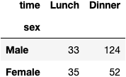
We can use .pivot_table() to represent the data clearer:
df_tips.pivot_table(index='sex', columns='time', aggfunc='size')
Other Example 1
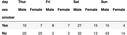
df_tips.pivot_table(index='smoker', columns=['day', 'sex'],aggfunc='size')
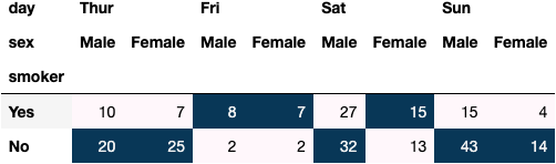
dfres = df_tips.pivot_table(index='smoker', columns=['day', 'sex'], aggfunc='size')
dfres.style.background_gradient()
Other Example 2
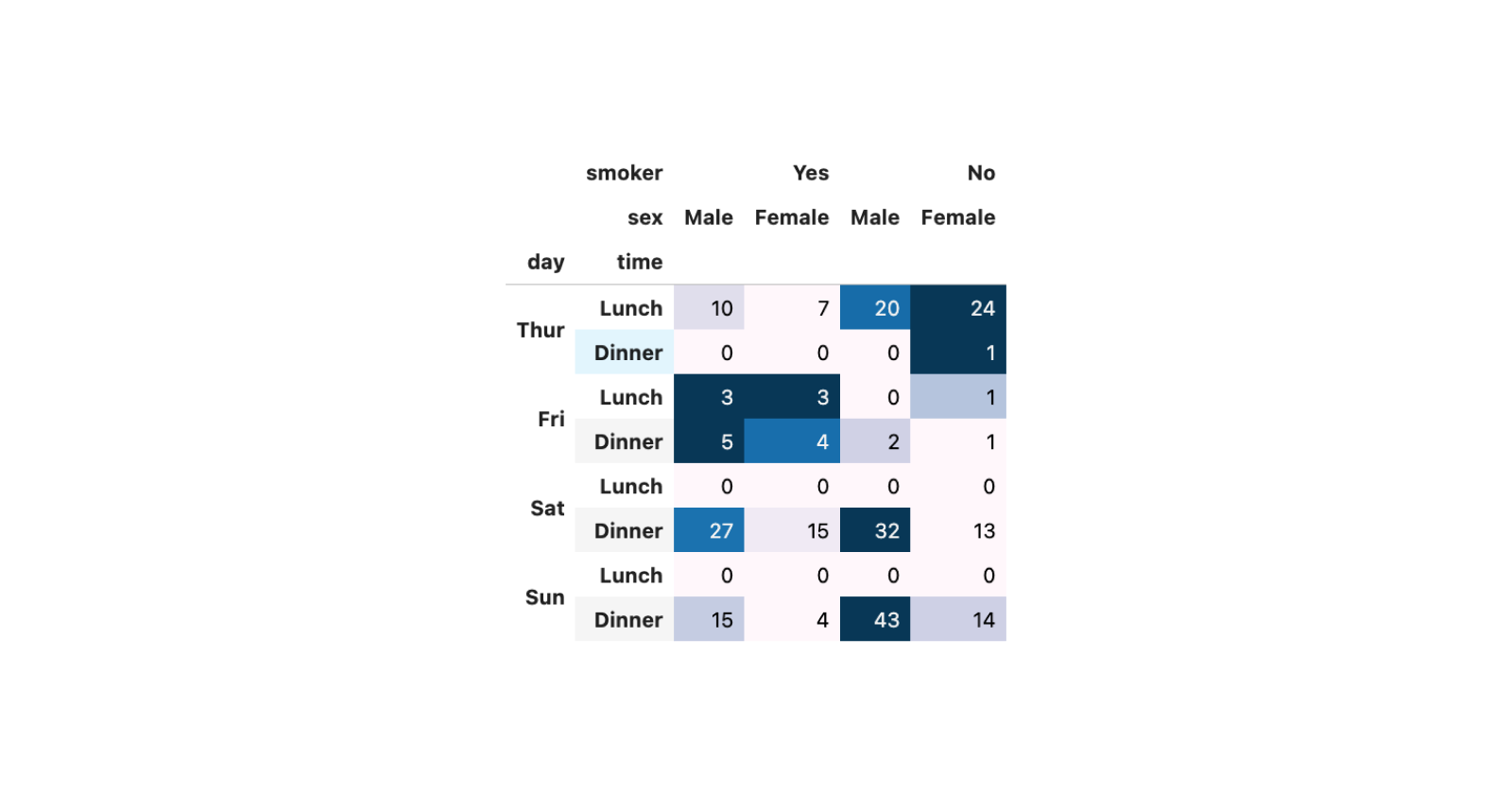
df_tips.pivot_table(index=['day', 'time'], columns=['smoker', 'sex'], aggfunc='size')
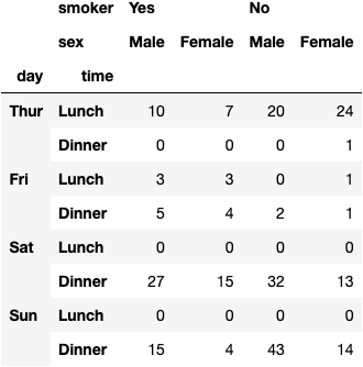
dfres = df_tips.pivot_table(index=['day', 'time'], columns=['smoker', 'sex'], aggfunc='size')
dfres.style.background_gradient()
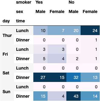
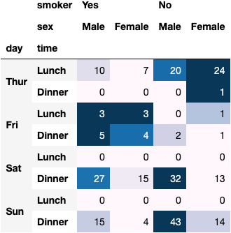
We can even choose the way we'd like to gradient colour the cells:
axis=1: the upper value between the columns of the same rowaxis=2: the upper value between the rows of the same column
dfres.style.background_gradient(axis=1)

This work is licensed under a Creative Commons Attribution-NonCommercial-NoDerivatives 4.0 International License.
About the author
I coach people to develop the Resolving Discipline that turns them into independent programmers.
Comments
Join the discussionNo comments yet. Be the first to comment.
Pandas
This series of tutorials shows you how to work with Pandas, a Python library used to work with data tables.