#05 | DateTime Object's Potential within Pandas, a Python Library
Learn how you can save vast amounts of time by applying the DateTime functionalities of Pandas. Instead of thinking about for loops.

I coach people to develop the Resolving Discipline that turns them into independent programmers.
© Jesús López
Ask him any doubt on Twitter or LinkedIn
Possibilities
Look at the following example as an aspiration you can achieve if you fully understand and replicate this whole tutorial with your data.
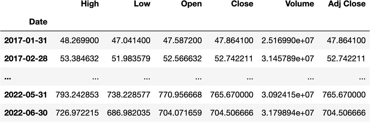
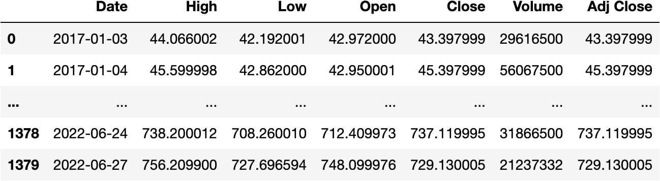
Let's load a dataset containing information on the Tesla Stock daily (rows) transactions (columns) in the Stock Market.
import pandas as pd

url = 'https://raw.githubusercontent.com/jsulopzs/data/main/tsla_stock.csv'
df_tesla = pd.read_csv(url, index_col=0, parse_dates=['Date'])
df_tesla

You may calculate the .mean() of each column by the last Business day of each Month (BM):
df_tesla.resample('BM').mean()
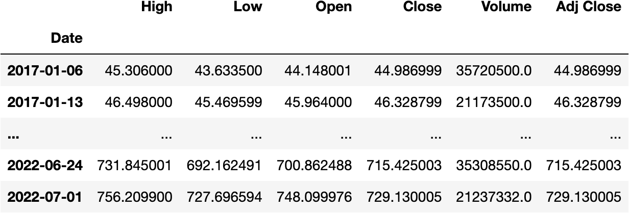
Or the Weekly Average:
df_tesla.resample('W-FRI').mean()
And many more; see the full list here.
Pretty straightforward compared to other libraries and programming languages.
It's not a casualty they say Python is the future language because its libraries simplify many operations where most people believe they would have needed a for loop.
Let's apply other pandas techniques to the DateTime object:
df_tesla['year'] = df_tesla.index.year
df_tesla['month'] = df_tesla.index.month
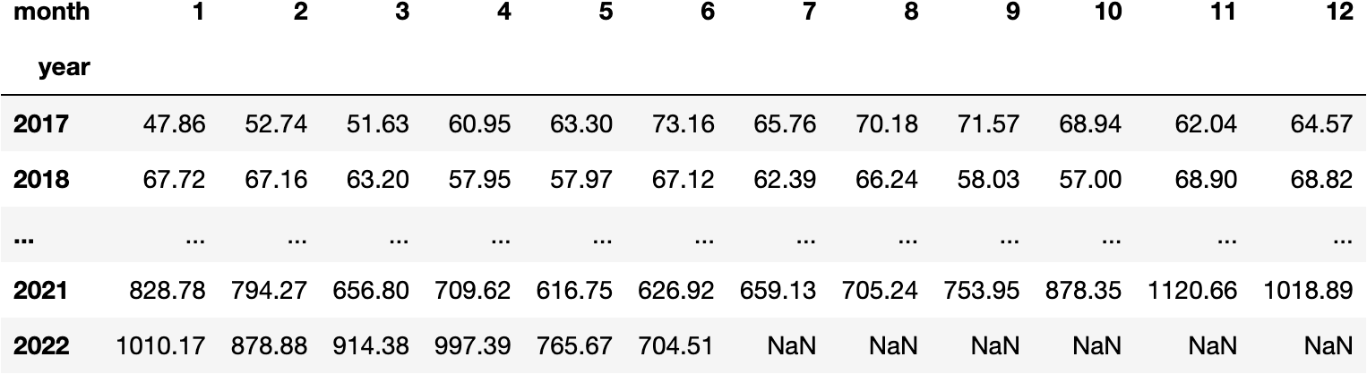
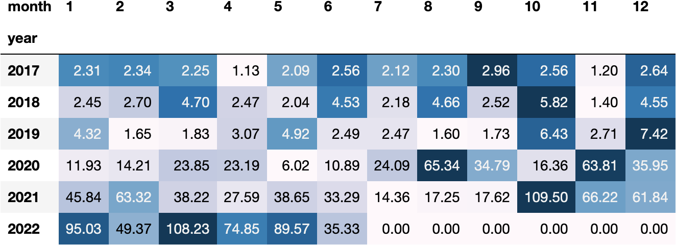
The following values represent the average Close price by each month-year combination:
df_tesla.pivot_table(index='year', columns='month', values='Close', aggfunc='mean').round(2)
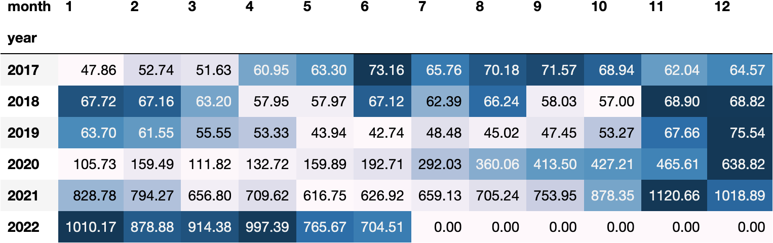
We could even style it to get a better insight by colouring the cells:
df_stl = df_tesla.pivot_table(
    index='year',
    columns='month',
    values='Close',
    aggfunc='mean',
    fill_value=0).style.format('{:.2f}').background_gradient(axis=1)

df_stl
And they represent the volatility with the standard deviation:
df_stl = df_tesla.pivot_table(
    index='year',
    columns='month',
    values='Close',
    aggfunc='std',
    fill_value=0).style.format('{:.2f}').background_gradient(axis=1)

df_stl
In this article, we'll dig into the details of the Panda's DateTime-related object in Python to understand the required knowledge to come up with awesome calculations like the ones we saw above.
First, let's reload the dataset to start from the basics.
df_tesla = pd.read_csv(url, parse_dates=['Date'])
df_tesla
Series DateTime
An essential part of learning something is the practicability and the understanding of counterexamples where we understand the errors.
Let's go with basic thinking to understand the importance of the DateTime object and how to work with it. So, out of all the columns in the DataFrame, we'll now focus on Date:
df_tesla.Date
0      2017-01-03
1      2017-01-04
          ...
1378   2022-06-24
1379   2022-06-27
Name: Date, Length: 1380, dtype: datetime64[ns]
What information could we get from a DateTime object?
- We may think we can get the month, but it turns out we can't in the following manner:
df_tesla.Date.month
---------------------------------------------------------------------------

AttributeError                            Traceback (most recent call last)

Input In [53], in <cell line: 1>()
----> 1 df_tesla.Date.month


File ~/miniforge3/lib/python3.9/site-packages/pandas/core/generic.py:5575, in NDFrame.__getattr__(self, name)
   5568 if (
   5569     name not in self._internal_names_set
   5570     and name not in self._metadata
   5571     and name not in self._accessors
   5572     and self._info_axis._can_hold_identifiers_and_holds_name(name)
   5573 ):
   5574     return self[name]
-> 5575 return object.__getattribute__(self, name)


AttributeError: 'Series' object has no attribute 'month'
Programming exists to simplify our lives, not make them harder.
Someone has probably developed a simpler functionality if you think there must be a simpler way to perform certain operations. Therefore, don't limit programming applications to complex ideas and rush towards a for loop, for example; proceed through trial and error without losing hope.
In short, we need to bypass the dt instance to access the DateTime functions:
df_tesla.Date.dt
<pandas.core.indexes.accessors.DatetimeProperties object at 0x16230a2e0>
Process the Month
df_tesla.Date.dt.month
0       1
1       1
       ..
1378    6
1379    6
Name: Date, Length: 1380, dtype: int64
We can use more elements than just .month:
Process the Month Name
df_tesla.Date.dt.month_name()
0       January
1       January
         ...
1378       June
1379       June
Name: Date, Length: 1380, dtype: object
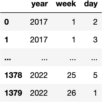
Process the Year, Week & Day
df_tesla.Date.dt.isocalendar()
Process the Quarter
df_tesla.Date.dt.quarter
0       1
1       1
       ..
1378    2
1379    2
Name: Date, Length: 1380, dtype: int64
Process the Year-Month for each Date
df_tesla.Date.dt.to_period('M')
0       2017-01
1       2017-01
         ...
1378    2022-06
1379    2022-06
Name: Date, Length: 1380, dtype: period[M]
Process the Weekly Period for each Date
df_tesla.Date.dt.to_period('W-FRI')
0       2016-12-31/2017-01-06
1       2016-12-31/2017-01-06
                ...
1378    2022-06-18/2022-06-24
1379    2022-06-25/2022-07-01
Name: Date, Length: 1380, dtype: period[W-FRI]
Time Zones
Pandas contain functionality that allows us to place Time Zones into the objects to ease the work of data from different countries and regions.
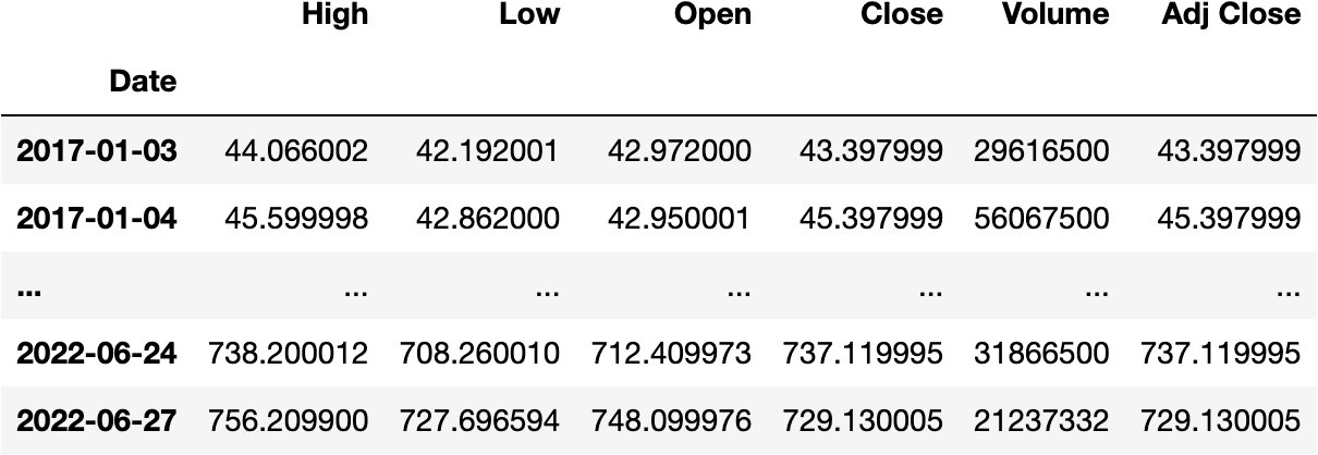
Before getting deeper into Time Zones, we need to set the Date as the index (rows) of the DataFrame:
df_tesla.set_index('Date', inplace=True)
df_tesla
We can tell Python the DateTimeIndex of the DataFrame comes from Madrid:
df_tesla.index = df_tesla.index.tz_localize('Europe/Madrid')
df_tesla

And change it to another Time Zone, like Moscow:
df_tesla.index.tz_convert('Europe/Moscow')
DatetimeIndex(['2017-01-03 02:00:00+03:00', '2017-01-04 02:00:00+03:00',
               '2017-01-05 02:00:00+03:00', '2017-01-06 02:00:00+03:00',
               ...
               '2022-06-22 01:00:00+03:00', '2022-06-23 01:00:00+03:00',
               '2022-06-24 01:00:00+03:00', '2022-06-27 01:00:00+03:00'],
              dtype='datetime64[ns, Europe/Moscow]', name='Date', length=1380, freq=None)
We could have applied the transformation in the DataFrame object itself:
df_tesla.tz_convert('Europe/Moscow')
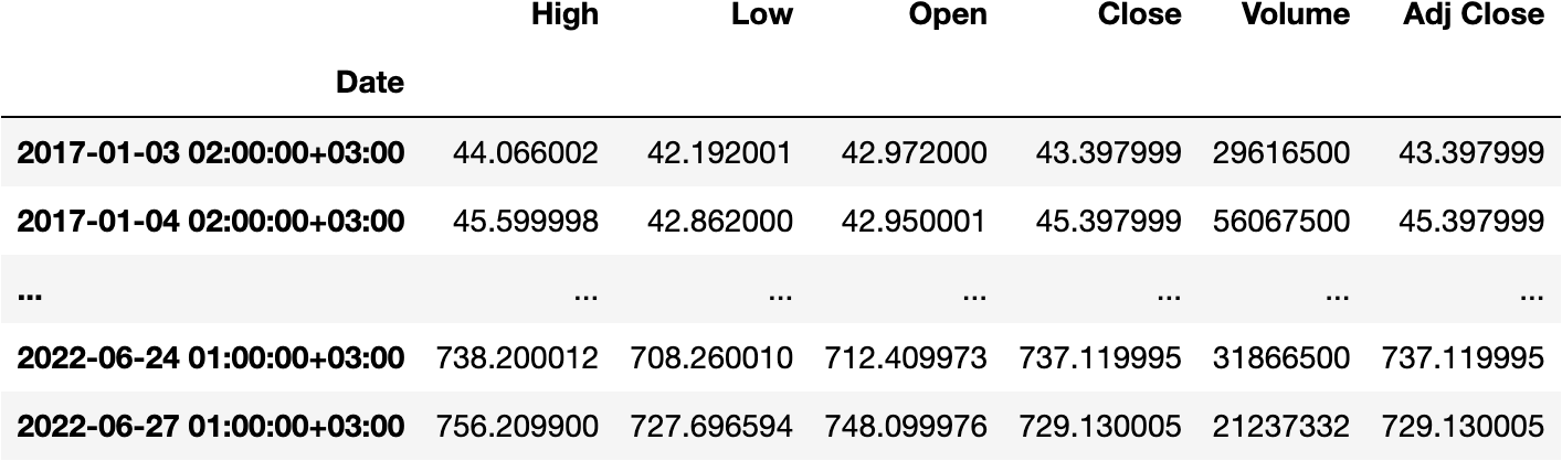
We can observe the hour has changed accordingly.
The Pandas Time Zone functionality is useful for combining timed data from different regions around the globe.
Summarising the Dates
To summarise, for example, the information of daily operations into months, we can apply different functions with each one having its unique ability (it's up to you to select the one that suits your needs):
.groupby().resample().pivot_table()
Let's show some examples:
Groupby
df_tesla.groupby(by=df_tesla.index.year).Volume.sum()
Date
2017     7950157000
2018    10808194000
2019    11540242000
2020    19052912400
2021     6902690500
2022     3407576732
Name: Volume, dtype: int64
The function .groupby() packs the rows of the same year:
df_tesla.groupby(by=df_tesla.index.year)
<pandas.core.groupby.generic.DataFrameGroupBy object at 0x1622eecd0>
To later summarise the total volume in each pack as we saw before.
An easier way?
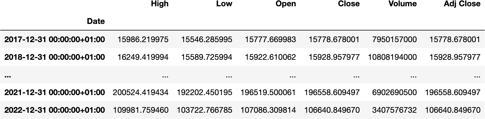
Resample
df_tesla.Volume.resample('Y').sum()
Date
2017-12-31 00:00:00+01:00     7950157000
2018-12-31 00:00:00+01:00    10808194000
2019-12-31 00:00:00+01:00    11540242000
2020-12-31 00:00:00+01:00    19052912400
2021-12-31 00:00:00+01:00     6902690500
2022-12-31 00:00:00+01:00     3407576732
Freq: A-DEC, Name: Volume, dtype: int64
We first select the column in which we want to apply the operation:
df_tesla.Volume
Date
2017-01-03 00:00:00+01:00    29616500
2017-01-04 00:00:00+01:00    56067500
                               ...
2022-06-24 00:00:00+02:00    31866500
2022-06-27 00:00:00+02:00    21237332
Name: Volume, Length: 1380, dtype: int64
And apply the .resample() function to take a Date Offset to aggregate the DateTimeIndex. In this example, we aggregate by year 'Y':
df_tesla.Volume.resample('Y')
<pandas.core.resample.DatetimeIndexResampler object at 0x16230abe0>
And apply mathematical operations to the aggregated objects separately as we saw before:
df_tesla.Volume.resample('Y').sum()
Date
2017-12-31 00:00:00+01:00     7950157000
2018-12-31 00:00:00+01:00    10808194000
2019-12-31 00:00:00+01:00    11540242000
2020-12-31 00:00:00+01:00    19052912400
2021-12-31 00:00:00+01:00     6902690500
2022-12-31 00:00:00+01:00     3407576732
Freq: A-DEC, Name: Volume, dtype: int64
We could have also calculated the .sum() for all the columns if we didn't select just the Volume:
df_tesla.resample('Y').sum()
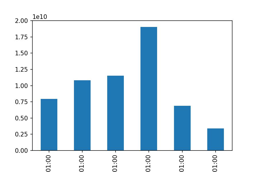
As always, we should strive to represent the information in the clearest manner for anyone to understand. Therefore, we could even visualize the aggregated volume by year with two more words:
df_tesla.Volume.resample('Y').sum().plot.bar();
Let's now try different Date Offsets:
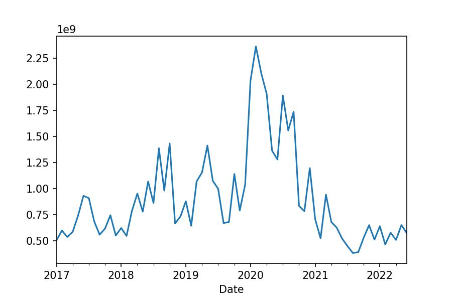
Monthly
df_tesla.Volume.resample('M').sum()
Date
2017-01-31 00:00:00+01:00    503398000
2017-02-28 00:00:00+01:00    597700000
                               ...
2022-05-31 00:00:00+02:00    649407200
2022-06-30 00:00:00+02:00    572380932
Freq: M, Name: Volume, Length: 66, dtype: int64
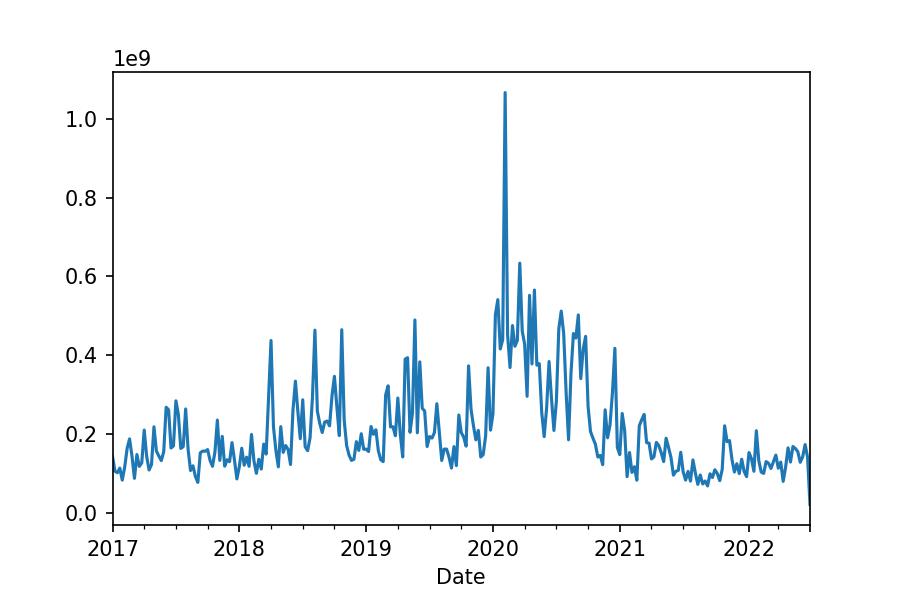
df_tesla.Volume.resample('M').sum().plot.line();
Weekly
df_tesla.Volume.resample('W').sum()
Date
2017-01-08 00:00:00+01:00    142882000
2017-01-15 00:00:00+01:00    105867500
                               ...
2022-06-26 00:00:00+02:00    141234200
2022-07-03 00:00:00+02:00     21237332
Freq: W-SUN, Name: Volume, Length: 287, dtype: int64
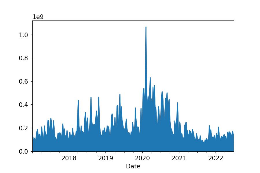
df_tesla.Volume.resample('W').sum().plot.area();
df_tesla.Volume.resample('W-FRI').sum()
Date
2017-01-06 00:00:00+01:00    142882000
2017-01-13 00:00:00+01:00    105867500
                               ...
2022-06-24 00:00:00+02:00    141234200
2022-07-01 00:00:00+02:00     21237332
Freq: W-FRI, Name: Volume, Length: 287, dtype: int64
df_tesla.Volume.resample('W-FRI').sum().plot.line();
Quarterly
df_tesla.Volume.resample('Q').sum()
Date
2017-03-31 00:00:00+02:00    1636274500
2017-06-30 00:00:00+02:00    2254740000
                                ...
2022-03-31 00:00:00+02:00    1678802000
2022-06-30 00:00:00+02:00    1728774732
Freq: Q-DEC, Name: Volume, Length: 22, dtype: int64
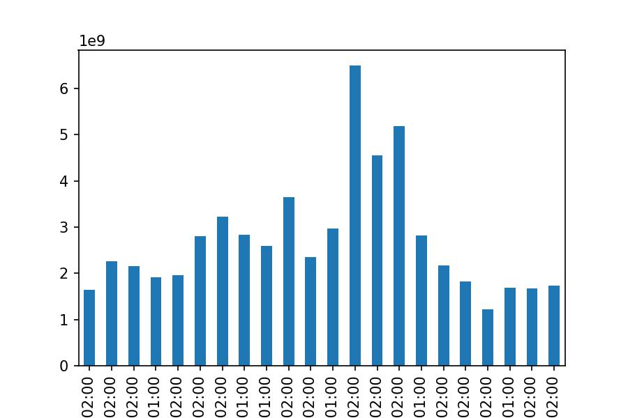
df_tesla.Volume.resample('Q').sum().plot.bar();
Pivot Table
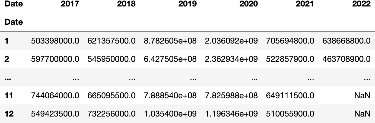
We can also use Pivot Tables for summarising and nicer represent the information:
df_res = df_tesla.pivot_table(
    index=df_tesla.index.month,
    columns=df_tesla.index.year,
    values='Volume',
    aggfunc='sum'
)

df_res
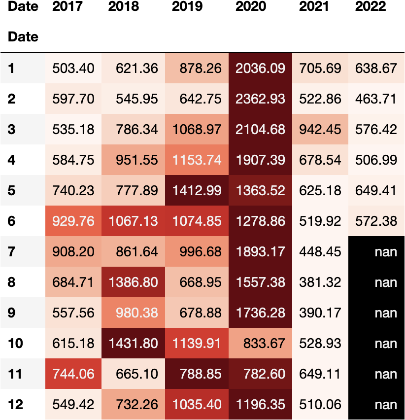
And even apply some style to get more insight on the DataFrame:
df_tesla['Volume_M'] = df_tesla.Volume/1_000_000

dfres = df_tesla.pivot_table(
    index=df_tesla.index.month,
    columns=df_tesla.index.year,
    values='Volume_M',
    aggfunc='sum'
)

df_stl = dfres.style.format('{:.2f}').background_gradient('Reds', axis=1)
df_stl

This work is licensed under a Creative Commons Attribution-NonCommercial-NoDerivatives 4.0 International License.